





Imagine your dashboard displays average request durations from two servers. The first handled few requests, the second many more. To obtain the overall average, adding the two averages and dividing by two is not enough: you must also account for the request count behind each number.
The same trap exists when two GPUs train a model on sequences of different lengths. Each card can compute a perfectly correct average on its own data, then contribute to a global calculation that no longer represents the chosen objective.
We will make this problem visible using a small model and synthetic data. We will compare a two-GPU computation with a single-GPU reference, then interrupt training to verify resumption. The goal is neither to beat a known model nor measure acceleration: we want to recover the gradient of an average over every valid token in the same training window.
The project requires no pretrained weights or external corpus. You can follow the reasoning with Python basics and a few average calculations; the executable workflow uses Docker and two GPUs. Reported numbers remain those of the r1 reference run. Additional small examples explain calculations rather than announce new model measurements.
The problem: an average of averages is biased
First, what do we want the model to learn?
A model has parameters, also called weights: numbers adjusted during training. For a data batch, it produces predictions that the program compares with expected answers. The loss summarizes error cost according to the chosen rule.
In this tutorial, loss consists of contributions from each supervised token. A token is a sequence unit represented by a numerical identifier in the program. For text, it might correspond to a word, part of a word, or a symbol; here, sequences are synthetic. “Supervised” means an expected answer actually contributes to loss at that position.
The gradient indicates how loss changes when parameters change slightly. It contains one derivative per parameter. Computing these derivatives is called backpropagation, or backward. An optimizer then uses gradients to modify weights. We will see both operations in the code: computing a gradient does not yet apply the update.
Our choice is precise: every supervised token counts equally in the window's average. A long sequence therefore contributes more terms than a short one. We are not aiming to give every sequence equal total weight.
Two processes, two token counts
A rank identifies a process participating in distributed computation. In our experiment, rank 0 works on one GPU and rank 1 on the other. Each has a copy of the same model but receives different sequences.
Return to the project's counterexample. The first rank processes 12 tokens and obtains a loss sum of 12. The second processes 36 tokens and obtains a loss sum of 108.
On mobile, scroll the table horizontally.
| Rank | Valid tokens | Loss sum | Local mean | Share of window tokens |
|---|---|---|---|---|
| 0 | 12 | 12 | 12 / 12 = 1 |
12 / 48 = 25 % |
| 1 | 36 | 108 | 108 / 36 = 3 |
36 / 48 = 75 % |
The mean of local means gives:
(1 + 3) / 2 = 2.
But the mean across all tokens gives:
(12 + 108) / (12 + 36) = 120 / 48 = 2,5.
We can also recover this result by weighting local means:
25 % × 1 + 75 % × 3 = 2,5.
What happened in the first calculation? The shorter rank received half the total weight even though it contains only a quarter of the tokens. Each rank-0 token weighs 1 / (2 × 12), versus 1 / (2 × 36) for a rank-1 token: the former weighs three times as much.
This is therefore not a rounding error. We changed the question: “what is the average across two ranks?” replaced “what is the average across all tokens?”
When ranks contain equal token counts, the formulas coincide. Identical local means can also hide the difference. That is why testing only balanced batches cannot detect the problem.
Where does DDP come in?
DistributedDataParallel, or DDP, synchronizes gradients across model copies. In the operation used here, aggregation corresponds to averaging across ranks. However, DDP does not know your objective is a per-token average, and it does not distribute inputs for you. Selecting sequences remains the application's responsibility, as the PyTorch DDP documentation explains.
The tutorial therefore prepares a correctly weighted loss on each rank before backward. DDP can then synchronize gradients without changing the intended global objective.
Prerequisites: Docker and two GPUs
The validated workflow requires Linux x86_64, Docker with Compose, NVIDIA Container Toolkit, and two 24 GiB RTX 3090 cards visible inside the container. Also allow 16 GiB of RAM and 16 GiB of disk space, excluding shared Docker layers.
VRAM is each graphics card's own memory. Two 24 GiB cards remain two separate memories: DDP places a model replica on each; it does not create a virtual 48 GiB card. CUDA runs computations on NVIDIA GPUs here. NCCL is the backend used for communication between GPU processes; this protocol does not validate a CPU or Gloo workflow instead.
In Docker, the gpu service runs preparation and simple checks. The dual service handles the two-process workflow. torchrun, which we will use later, launches these processes inside the container.
The setup.sh script creates directories and writes only UID/GID to .env. These identify the host user and group. outputs/ receives measurements; artifacts/ receives checkpoints, saved states for resuming training.
There are no pretrained weights or external data to acquire, so acquire checks an empty acquisition. This does not mean Docker image building requires no resources; experimental data will be generated by the project itself.
Extract the archive and place your terminal at its root. Run every following command from this same directory. Start by building images and checking access to one GPU, then both:
sh scripts/setup.sh
docker compose config --quiet
docker compose build acquire gpu dual
docker compose run --rm acquire python scripts/acquire.py --config configs/minimum.yaml
docker compose run --rm gpu python scripts/check_environment.py --config configs/minimum.yaml
docker compose run --rm dual python scripts/check_environment.py --config configs/minimum.yaml --dual
docker compose config --quiet checks Compose configuration. Environment scripts actually initialize CUDA and check visible cards: a GPU's presence on the host does not demonstrate Docker access.
Both environment checks must pass before continuing. On failure, fix that issue before running torchrun; the official NVIDIA Container Toolkit guide describes Docker integration.
Existing Docker layers may shorten a build. They do not change the normalization formula we will compare.
Checking the program before distributed computation
Before launching both processes, run the public tests. They cover the project's normalization and resume functions:
docker compose run --rm gpu python -m pytest -q
This follows the same logic as testing a shopping-cart calculation before trying a complete order: first we verify the functions, then their behavior in the real workflow.
A passing result for this suite does not replace the numerical comparison with the single-GPU reference. Nor does it replace the interruption-and-resume test. Those checks come next and answer different questions.
Data: deliberately creating an imbalance
Short sequences on one side, long ones on the other
The corpus contains 1,024 training sequences, 128 validation sequences, and 256 test sequences. In each training window, rank 0 receives sequences of 16 to 64 tokens, while rank 1 receives sequences of 65 to 128 tokens.
This imbalance is intentional. It forces the program to distinguish the number of sequences from the number of tokens. Even with the same number of sequences on each card, the two ranks do not carry the same amount of supervision.
A microbatch is the small batch handled in one pass through the model. An accumulation window groups several microbatches whose gradients are added before a single weight update. Here, each window contains two microbatches per rank.
The following plan selects the identifiers of those sequences. It does not yet calculate loss, move anything to GPUs, or build padding arrays itself.
def make_rank_batches(rows, config):
    pools = [
        [
            r["id"]
            for r in rows
            if r["split"] == "train" and (len(r["tokens"]) <= 64) == (rank == 0)
        ]
        for rank in range(2)
    ]
    rng = random.Random(config["seed"] + 10)
    plan = []
    for step in range(config["updates"]):
        selected = [
            rng.sample(pool, config["accumulation"] * config["batch_size_per_rank"])
            for pool in pools
        ]
        plan.append(
            [
                [
                    ids[i : i + config["batch_size_per_rank"]]
                    for i in range(0, len(ids), config["batch_size_per_rank"])
                ]
                for ids in selected
            ]
        )
    return plan
Reading the plan as a Python data structure
The pools variable contains two lists of identifiers. The filter keeps only train rows. The expression (len(r["tokens"]) <= 64) == (rank == 0) places short sequences in the first group and long ones in the second. The bounds 16 and 128 belong to the prepared corpus; this function uses only the cutoff at 64.
The random.Random(config["seed"] + 10) generator isolates selection for this plan. With identical data, list order, and configuration, its choices can be reproduced.
For each update, rng.sample takes accumulation × batch_size_per_rank identifiers from each group. The ids[i : i + batch_size_per_rank] slicing then distributes them into microbatches. The structure reads as follows: plan[step][rank][microbatch] gives the list of identifiers to process.
Within one window, selection is without replacement: an identifier is not selected twice for the same rank. Because the groups are disjoint, it is not shared between ranks either. In the next window, however, the same identifier may return. The code does not permanently remove items from the group. That is how random.sample behaves when used for each new window.
We therefore do not necessarily traverse the whole corpus once before seeing an example again. The plan is defined by updates, not by the implicit assumption of a complete pass without repetition.
Two kinds of “padding” not to confuse
Token padding extends short sequences to form a rectangular array. To visualize the idea with a miniature example separate from the corpus, [7, 4, 9] and [5, 2] can become [7, 4, 9] and [5, 2, PAD]. The array has six slots but only five original tokens. The added slot must not increase the loss denominator.
Sampler padding refers to another issue: completing a data plan by repeating some identifiers to balance processes. Here, the plan introduces no such duplicates between ranks within a window. The token imbalance remains visible rather than being hidden.
Now build the corpus, the plan, and the single-GPU reference:
docker compose run --rm gpu python -m ddp_tokens.cli prepare --config configs/minimum.yaml
docker compose run --rm gpu python -m ddp_tokens.cli reference --config configs/minimum.yaml
docker compose run --rm gpu python -m ddp_tokens.cli check-loss --config configs/minimum.yaml
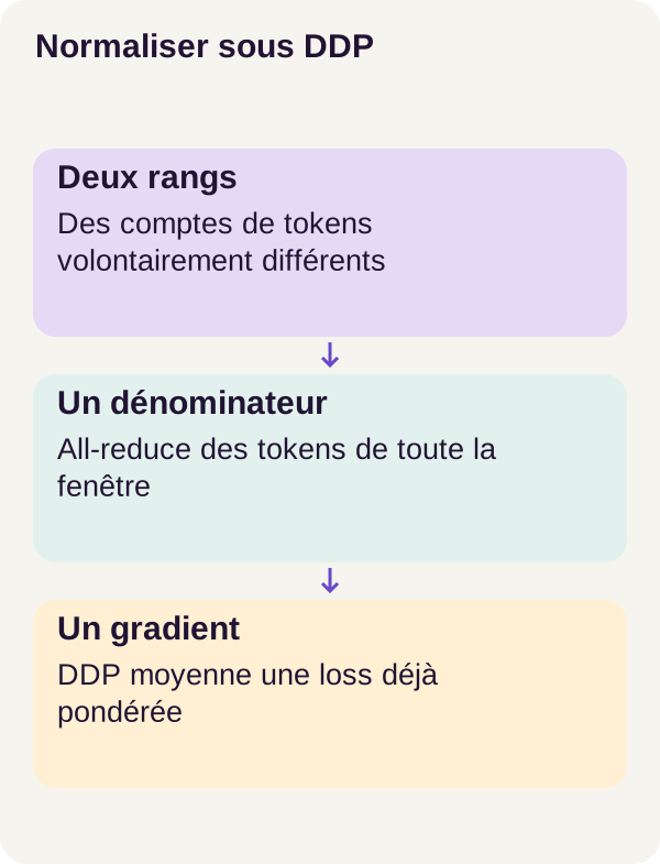
prepare fixes the sequences and windows. reference starts from the same initial state as the distributed comparison and serves as the control computation. check-loss exposes the two counterexample values, 2 and 2.5, before any run with torchrun.
At this point, we have the data and a result to compare against. What remains is to understand how to weight local losses to recover it.
The central calculation: the global denominator
One denominator for the whole window
Let us name the quantities once so we can read the formula:
W is the number of ranks, therefore 2 in this project. S_r is the sum of losses for rank r across its whole window. N_r is its number of supervised tokens. Finally, N = sum of N_r is the total number of supervised tokens for both ranks across the two microbatches.
The intended objective is:
L = (S_0 + S_1) / N.
It might be tempting to have each rank compute S_r / N. But DDP then averages gradients between the two processes: that would add a division by 2 that we do not need.
Each rank therefore uses:
L_r = W × S_r / N.
After DDP averaging, the W factor cancels out:
(1 / W) × sum_r gradient(W × S_r / N) = gradient(sum_r S_r / N).
Here, “gradient” means derivatives with respect to the weights. The reasoning relies on a denominator fixed by the window data, independent of the weights, and on the gradient average used by this DDP. Multiplying by W is not intended to “learn twice as fast”: it compensates for a division already present in aggregation.
In our counterexample, W / N = 2 / 48 = 1 / 24. Rank 0 therefore uses 12 / 24 = 0.5 and rank 1 uses 108 / 24 = 4.5. The average of these contributions is (0.5 + 4.5) / 2 = 2.5.
These two local scalars are no longer the local means 1 and 3. That is normal: they are prepared for aggregation. Confusing them with an average metric already computed over the whole corpus would make logs misleading.
Count before backpropagating
def global_token_loss(local_sum, global_count, world_size):
    if global_count <= 0:
        raise ValueError(
            "No supervised token in the global accumulation window; all ranks must skip or stop together"
        )
    return local_sum * (world_size / global_count)


def global_count(local_count, device):
    count = torch.tensor(local_count, device=device, dtype=torch.long)
    dist.all_reduce(count, op=dist.ReduceOp.SUM)
    return int(count)
global_token_loss receives a sum, not an already averaged loss. It multiplies it by the shared world_size / global_count factor. Providing a local average instead would alter the weighting a second time.
The global_count function turns the local count into an integer tensor on the device in use. A tensor here is simply a numeric value that PyTorch can manipulate and communicate. dist.all_reduce(..., SUM) adds the counts and leaves the total in the tensor on every rank: 12 and 36 become 48 in both processes. int(count) retrieves that total as a Python integer. The PyTorch collectives documentation describes this in-place operation.
A collective is a communication in which the processes in the group participate together. The count is therefore not sent to a single “leader” that keeps the result: both ranks need the same denominator before backward.
Keep two separate operations in mind: the program first adds token counts, then DDP synchronizes gradients. The code above does not automatically synchronize a global loss metric.
What if the window contains no supervised token?
An average over zero tokens is undefined. The global_count <= 0 branch therefore raises an error rather than manufacturing a zero loss.
In this project, ranks collectively reject the same window. The function alone does not, however, establish all coordination: the caller must have computed the same global count and ensure the processes follow a compatible path.
Imagine two workers that must meet at an exchange step. If one alone decides to leave the loop while the other is still waiting for that exchange, the latter may remain blocked. A local condition must therefore not cause an isolated skip of a collective or a backward expected by the other ranks.
A locally empty rank is not the same as a globally empty window. If other ranks have supervision, the global denominator can be positive. Adapting the project to this case would require testing correct participation in computation and communication; the N <= 0 guard alone does not prove that every locally empty case is handled.
What check_loss() verifies exactly
def check_loss(config):
    local_sums = [12.0, 108.0]
    counts = [12, 36]
    wrong = sum(s / n for s, n in zip(local_sums, counts)) / 2
    correct = sum(global_token_loss(s, sum(counts), 2) for s in local_sums) / 2
    assert correct == 2.5 and wrong == 2.0
    return {
        "local_tokens": counts,
        "local_loss_sums": local_sums,
        "mean_of_means": wrong,
        "global_mean": correct,
    }
wrong reproduces the average of averages: 2. correct applies the weighted formula and then averages across the two ranks: 2.5. The config parameter is not used in this small check; the values are deliberately fixed in the function.
The test runs on Python numbers. It does not run a neural network, backward pass, or DDP communication. It verifies the arithmetic identity; the actual gradient comparison comes in the GPU protocol.
The wrong variant must remain wrong. It acts as a negative control: a test that can accept the correct formula but cannot reject the incorrect one would not protect the mechanism under study. An additional division by the number of microbatches would not correct this weighting.
Why identical loss is not enough to prove identical gradients
Here is an educational example independent of the r1 model, with one parameter θ and squared error.
Rank 0 has 12 targets equal to +1: its loss sum is 12 × (θ − 1)². Rank 1 has 36 targets equal to −1: its sum is 36 × (θ + 1)².
At θ = 0, every token has a loss of 1. Both methods therefore display an average loss of 1. Looking only at that number, we see no difference.
But the derivative of (θ − 1)² is 2 × (θ − 1), or −2 at that point. The derivative of (θ + 1)² is +2. The average of averages then produces a gradient (-2 + 2) / 2 = 0. The global average produces (12 × -2 + 36 × 2) / 48 = 1.
Same displayed loss, different gradients. This is exactly why our validation compares gradients themselves, not just two loss values in a log.
Accumulation: include forward and backward
Two microbatches, one update
Rather than calculating a whole window in one pass, we process its microbatches successively. Each backward() call adds its contribution to gradients already present. The Tensor.backward documentation describes this accumulation: old gradients must therefore be cleared at the right time, not after every microbatch.
During this window, weights must not be updated between microbatches. Otherwise, contributions would be calculated from different model states and would no longer represent the gradient of the same sum.
The forward calculates predictions from inputs. The backward calculates loss derivatives. no_sync() removes neither calculation: it postpones gradient synchronization between ranks for intermediate microbatches.
def accumulate(model, batches, mapping, rank, denominator, world, wrong=False):
    model.zero_grad(set_to_none=True)
    local_n = sum(len(mapping[i]["tokens"]) for micro in batches for i in micro)
    for index, ids in enumerate(batches):
        # The context deliberately includes the forward as well as the backward.
        context = (
            model.no_sync() if index < len(batches) - 1 else contextlib.nullcontext()
        )
        with context:
            tokens, labels = padded(ids, mapping, rank)
            summed = loss_sum(model(tokens), labels)
            loss = (
                summed / local_n
                if wrong
                else global_token_loss(summed, denominator, world)
            )
            loss.backward()
    return local_n
Following each line's responsibilities
model.zero_grad(set_to_none=True) removes gradients from the previous window. This instruction is placed before the loop so that the next two backward passes can contribute to the same accumulation.
local_n counts the original tokens in this rank's sequences across the whole window. mapping retrieves a sequence from its identifier. The global denominator already arrives in the denominator parameter: accumulate() does not obtain it by calling global_count() in this loop.
For each microbatch, padded() prepares inputs and supervision labels. model(tokens) performs the forward pass, then loss_sum() returns the sum of losses for retained positions. The small network, padding, and this loss function belong to the complete project; the article excerpts focus on normalization and accumulation.
The wrong=True choice divides each microbatch sum by local_n. After the microbatches are added, this becomes the rank's local average. DDP then averages it across ranks: that is exactly the incorrect reference the test must detect.
On the correct path, each microbatch instead uses the same global count for the window. It is normalized neither by its own length nor by a denominator recalculated for that pass alone.
Finally, the function returns local_n. It contains no call to optimizer.step(): weight updates belong to the surrounding training loop. The project adds no new division when that update occurs.
Why put forward inside no_sync()?
For the first microbatch, context is model.no_sync(). For the last one, it is contextlib.nullcontext(), a context that changes nothing. DDP synchronization is therefore active on the final pass.
The subtle point is the scope of with: both forward and backward must be inside it. Surrounding only loss.backward() is not enough to suppress synchronization as intended. This is an explicit requirement in the no_sync() documentation.
At the end of the final backward pass, accumulated contributions take part in synchronization. This is a logical synchronization point for the window; it does not mean all gradients necessarily fit in a single network message.
Working through accumulation by hand
Let us split the 12/36 counterexample into two fictional microbatches per rank. This table illustrates the calculation; these are not batch lengths captured in r1.
On mobile, scroll the table horizontally.
| Rank | Microbatch | Valid tokens | Loss sum | Contribution with W / N = 2 / 48 |
|---|---|---|---|---|
| 0 | First | 4 | 4 | 4 / 24 ≈ 0.1667 |
| 0 | Second | 8 | 8 | 8 / 24 ≈ 0.3333 |
| 1 | First | 12 | 36 | 36 / 24 = 1.5 |
| 1 | Second | 24 | 72 | 72 / 24 = 3 |
Rank 0's two contributions total 0.5; rank 1's total 4.5. Their average remains 2.5. Splitting into microbatches has not changed the definition of the average.
Dividing each contribution again by accumulation = 2 would produce 1.25 after aggregation and would also halve the gradient. The global window denominator had already accounted for all four microbatches.
The rule is therefore not “never divide by the number of microbatches.” It is: do not add a division already contained in the chosen normalization. A recipe that starts from equal-sized microbatch averages must be reasoned about differently from this one, which starts from sums and a global count.
Running the stop, continuous workflow, and resume
We can now launch the three distributed runs: a stop at step 50, continuous training to 100, then a resume from 50 to 100.
docker compose run --rm dual torchrun --rdzv-backend=static --master-addr=127.0.0.1 --master-port=29500 --nnodes=1 --nproc-per-node=2 -m ddp_tokens.train --config configs/minimum.yaml
docker compose run --rm dual torchrun --rdzv-backend=static --master-addr=127.0.0.1 --master-port=29500 --nnodes=1 --nproc-per-node=2 -m ddp_tokens.train --config configs/minimum.yaml --continuous
docker compose run --rm dual torchrun --rdzv-backend=static --master-addr=127.0.0.1 --master-port=29500 --nnodes=1 --nproc-per-node=2 -m ddp_tokens.train --config configs/minimum.yaml --resume artifacts/checkpoints/step-0050
Run these commands one after another. --nnodes=1 describes one compute node, and --nproc-per-node=2 launches two processes. Static rendezvous at 127.0.0.1, port 29500, coordinates them locally. This port is not a business API port. The torchrun documentation explains the roles of the launcher and ranks.
The workflow without an extra option creates the planned stop at 50. --continuous produces the control run at 100 updates. --resume artifacts/checkpoints/step-0050 loads the interrupted state to continue the same workflow to 100.
A checkpoint is more than a weights file
Think of an interrupted data-processing job: retaining its partial result without knowing which items have already been read is not enough to resume in the right place. Training needs the same continuity.
The project's shared checkpoint contains the model, optimizer, configuration, and data lock. This lock identifies the expected data; it must not be confused with a lock that prevents two processes from entering a critical section.
Each rank also retains its random state, rank, and history. The program preserves sampler history, namely the mechanism used to select sequences. Resumption must recover both the weights and the continuation of the data workflow.
A seed initializes a pseudorandom generator. Its current state indicates where it is after selections already made. Resetting only the initial seed can restart the sequence of selections instead of continuing from the stop point. The PyTorch note on reproducibility helps distinguish random control from guarantees across environments.
The resume shown here occurs at an update boundary defined by the protocol. It does not demonstrate recovery from an arbitrary stop in the middle of a backward pass or communication.
Measurements to read before the results
Three questions, three checks
The first question is: does the DDP gradient match the single-GPU gradient? The project concatenates gradient values into a vector, then compares that vector with the reference obtained from the same initial state and the same tokens. The test covers 282,628 values, with tolerances atol=1e-6 and rtol=1e-4. This number describes compared components, not corpus size.
The second question is: does resumption recover the same parameters as continuous training? We then compare weights at step 100, not the gradients from the initial check. A correct formula and correct resumption are two distinct properties.
The third question is: what does the model trained on the test data achieve? The workflow performs 100 updates with SGD, in FP32, and with accumulation of two microbatches per rank. SGD is the optimizer used to apply gradients. FP32 means calculations use 32-bit floating-point numbers. The final test covers 256 sequences and 18,231 valid tokens.
Test token loss is an average loss per token. It is not a success percentage. Token accuracy measures the proportion of correctly predicted tokens among evaluated positions; it does not mean the same proportion of complete sequences is correct.
How to read numerical tolerances
An absolute tolerance bounds small differences, especially near zero. A relative tolerance adjusts to the magnitude of the reference value. The convention described for torch.allclose is, component by component:
abs(gradient_DDP - gradient_reference) <= atol + rtol × abs(gradient_reference).
With our tolerances, a reference equal to 0 allows a difference of up to 0.000001. A reference equal to 1 allows 0.000001 + 0.0001 = 0.000101. These are examples of reading the thresholds, not published components of the r1 gradient.
Why not require zero everywhere? The order of operations can differ between single-GPU and distributed computation. Yet additions in finite precision are not perfectly associative. The PyTorch note on numerical accuracy reminds us that a mathematical identity does not guarantee bit-for-bit equality between two calculation paths.
The proper check applies tolerances to every component. Maximum absolute error summarizes the largest difference, but does not by itself replace this complete comparison.
Reading the workflow report
Calculate the evaluation:
docker compose run --rm gpu python -m ddp_tokens.cli evaluate --config configs/minimum.yaml
The following values are local measurements observed in the r1 workflow. They do not predict the quality of another architecture, real data, another optimizer, or training across several nodes.
On mobile, scroll the table horizontally.
| Observed check | Result |
|---|---|
| Maximum absolute error, correct normalization | 3.73e-8 |
| Correct normalization within tolerances | Yes |
| Maximum absolute error, average of averages | 0.02157 |
| Incorrect normalization within tolerances | No |
| Maximum parameter difference, resumed vs. continuous | 0 |
| Test token loss | 1.31525 |
| Test token accuracy | 36.22% |
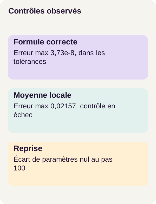
Correct normalization recovers the reference within tolerances, with a maximum absolute error of 3.73e-8. The average of averages fails the same check, with a maximum error of 0.02157. We therefore have both an accepted case and a deliberately introduced error that is actually detected.
The resume test answers another question: the maximum difference between resumed parameters and those from the continuous workflow is 0 at step 100. Preserving sampler history and random generators per rank is part of this resumption. The zero does not contradict the small single-GPU/DDP gradient difference: the two comparisons concern neither the same objects nor the same workflows.
The two ranks also reject a window with zero supervised tokens. This check complements the normal path: it verifies that a global absence of supervision is not treated as a valid average.
Finally, a test loss of 1.31525 and token accuracy of 36.22% do not demonstrate a business gain. The tutorial's central result is parity for the selected calculation. It is neither a model ranking nor a measure of two-GPU acceleration.
Exact resumption establishes the mechanism in this protocol. It does not prove the robustness of resuming a preempted run at any instant on distributed infrastructure.
What we learned
An average begins with a question: which unit should count as much as every other? Here, the answer is the supervised token. An average of rank-level averages assigns those tokens different weights when their counts differ.
DDP synchronizes gradients but does not know that intent. The world_size / global_count factor prepares local contributions so their average matches the intended gradient. The number of GPUs is not a coefficient to add or remove by habit: you must follow the divisions actually performed.
Accumulation does not change the objective. It splits the calculation into microbatches, with a denominator covering the whole window and weights unchanged between its passes. no_sync() postpones synchronization; it replaces neither token counting nor backward.
Finally, a checkpoint must make it possible to resume the trajectory, not merely reload a model. Future data, optimizer state, and random generators are also part of that continuity.
Exercise: form a hypothesis before the command
Rank 0 keeps 12 valid tokens. Rank 1 moves from 12 to 36 tokens, without changing the distribution of per-token losses we want to compare. Before running the program, predict what happens to the average of averages and the global average. Which one gives too much weight to the short rank?
To make your calculation explicit, let us use the educational assumption of a loss of 1 per token on rank 0 and 3 per token on rank 1, before and after the change. This assumption serves the manual calculation; the exercise gradients are those produced by its execution.
With 12 tokens on each rank, the sums are 12 and 36. Both averages produce 2. When the second rank moves to 36 tokens, its sum becomes 108: the average of averages remains 2, while the global average becomes 2.5.
The average of averages therefore does not see that the group with the highest loss now contains three times as many tokens. The short rank retains half the weight instead of a quarter.
Also write your prediction about normalization: should you change W, change N, or divide a second time by the number of microbatches? Both ranks remain present, so W remains 2; it is the global token count that changes.
Then run the workflow exercise:
docker compose run --rm gpu python -m ddp_tokens.cli exercise --config configs/exercise.yaml
Compare the supplied calculations and gradients with your hypothesis. Do not expect a 0.5 loss error to automatically produce a 0.5 gradient difference: a function value and its derivative are two different objects.
Keep the failure of the incorrect variant as a non-regression check. The purpose is not to make every mode pass by relaxing thresholds, but to verify that a future code change does not make incorrect weighting invisible.
Adapting the model and preparing for production
Choose the unit before copying the formula
In another project, the weighting unit might be a sequence, an example, a document, or a business cost. Giving every document the same total weight regardless of its length is not the same as giving equal weight to each of its tokens. Both choices can meet different needs; you must state which one is being trained.
The code's counter adds len(mapping[i]["tokens"]) here. That is consistent with this corpus's supervised tokens. This shortcut is not universal. In another training run, some input positions may be excluded from loss: an unsupervised prompt, ignored labels, or shifted targets. You must count positions that actually contribute to the objective, not merely input length.
As a general reference, CrossEntropyLoss documents ignored labels and the effects of weighting on reduction. That does not replace the definition of loss_sum() in your own application. Adding class weights or a regularization term also requires rederiving the normalization for each term, rather than mechanically applying the same denominator to the entire loss.
The formula shown also assumes the DDP aggregation of the reference workflow. A custom communication strategy, a variable number of participants, or ranks that no longer perform the same number of passes require the assumptions and tests to be revisited.
Testing an adaptation without changing the control
Keep the reference workflow, then work in a copy to modify the corpus or model. Always compare gradients obtained from the same initial state and the same supervised positions. Deliberately introduce unequal sizes: a test containing only identical counts can let the error studied here pass.
Check a globally empty window separately from branches where only one rank has no supervision. Do not conclude a branch is safe because the normal path's algebra is correct: you must also verify the order in which processes participate in communications.
What the demonstration does not provide
A distributed production deployment requires robust rendezvous between processes, timeouts, a recovery policy, logs and metrics per rank, preemption handling, multi-node tests, and a data strategy.
In particular, it must be possible to determine which rank failed, which step it had reached, and which consistent state can be restored. These are additional requirements, not automatic consequences of the zero difference observed at step 100. The demonstration on one host does not claim to cover them.
Troubleshooting and cleanup
The dual check fails. Do not run torchrun yet. Verify that two GPUs are exposed to the container and that each process selects its own card. Repair the environment before changing the training formula.
The processes appear stuck. Compare their latest messages and the order of collectives. One rank must not skip all_reduce alone, or a backward pass in which the other still participates. Unequal token counts are expected here; an incompatible number of communication steps is a different problem.
Gradient parity fails. First inspect the global count for the entire window, then verify that loss_sum() returns a sum, that no_sync() includes forward and backward, and that no extra division is applied. Also compare the initial state and data used by both paths.
The model reloads, but resumption differs. Reloading weights does not demonstrate complete resumption. Also examine the optimizer, configuration, data lock, position in the plan, and random states per rank before attributing the difference to DDP.
After your observations, generate the figure, check checkpoints, preview cleanup, and stop services:
docker compose run --rm gpu python lesson/figures/plot.py
docker compose run --rm gpu python scripts/check_checkpoints.py
docker compose run --rm gpu python scripts/clean.py --scope generated --dry-run
docker compose down --remove-orphans
Cleanup deliberately remains in --dry-run mode: it shows what would be affected without performing deletion. Examine that preview before making any decision to erase data. The final command stops this project's Compose services; it is not a request to purge your whole Docker environment.
Primary sources
The following links let you explore the mechanisms further. They do not replace the ZIP files and settings needed to reproduce r1; documentation references are not an additional record of executed versions.
- PyTorch 2.8 — DistributedDataParallel: replicas, gradient aggregation, and the scope of
no_sync(). - PyTorch — distributed collectives: the role of collective communications and
all_reduce. - NVIDIA Container Toolkit — installation guide: exposing GPUs to containers.
For reading the calculations: accumulation with Tensor.backward, torch.allclose tolerances, numerical accuracy, and CrossEntropyLoss reductions.
To understand processes and their state: the torchrun launcher, PyTorch reproducibility, and sampling without replacement with random.sample.