





You are developing a feature that turns a request into data your application can use. For example: find a product reference, a quantity, and a category, then return them as JSON. So far, the need resembles a conventional API. The difference is that a language model produces the response.
When you run it on your machine, you find several files for the same model: Q4_K_M, Q8_0… Which should you choose? Will the larger one necessarily be more reliable? Will the more compact one be accurate enough to power your application?
We will examine two measurement campaigns carried out with Qwen2.5 7B, in two quantized versions. The goal is not to crown a universal winner: it is to learn how to read the results, understand what a test checks, and connect those observations to a development need.
The central question is very concrete: is an answer that keeps a quantity but omits part of the product reference usable by your code?
Being able to read Python, handle JSON, and use Docker is enough to follow the explanations. We are not retraining a model. The execution path presented later nevertheless assumes you have the Lab and the experiment files: it is not a standalone installation from a blank machine.
Two campaigns using the same protocol
First, what does "quantizing a model" mean?
A model contains numerical values, called weights or parameters, which take part in its calculations. Quantization represents those values with reduced precision to make them take up less space. This is one way to use models with less memory. The Hugging Face guide to quantization presents this principle and its trade-offs.
To picture it, think of rounding: keeping 0.12 rather than 0.123456 retains an approximation but loses information. This is an analogy, not the formula used by this experiment's files. Actual methods encode groups of values and additional information.
In this comparison, the two names refer to different quantization recipes:
| Variant | What to keep in mind when reading the experiment |
|---|---|
Q4_K_M |
A recipe from the 4-bit quantization family, with a mix of precisions depending on the weights. Do not read this name as "exactly 4 bits for every parameter, with no other information." |
Q8_0 |
An 8-bit quantization recipe that keeps a finer representation of weights than lower-precision formats. This name is not a guarantee of success for every request. |
The Qwen documentation on llama.cpp explains weight quantization and type mixes. The llama.cpp quantization tool documentation describes the available variants.
Above all, keep the difference in mind between the precision of stored numbers and the correctness of an answer expected by your application. Our experiment measures the latter in a specific setting; it does not allow the two to be confused.
The model, the file, and the engine have different roles
Qwen2.5-7B-Instruct is the model. 7B indicates its size class, roughly seven billion parameters, and Instruct refers to a version adapted to following instructions. Its official model card at the revision used documents the distributed model.
GGUF is the file format: it contains the weights and metadata needed to load them. It is neither the model name nor, by itself, a quantization level. The GGUF specification describes this role.
llama.cpp is the engine that loads these files and runs the model. Using an already trained model to produce an answer is called inference. In our path, a Python program sends requests to a local llama.cpp server; the server documentation presents this interface.
What stays the same between the two variants
The campaigns compare Q4_K_M and Q8_0 from the same model, at the same revision, in a locked llama.cpp image. Here, "locked" means keeping an identified version rather than automatically retrieving the latest available one.
The protocol specifies 80 synthetic cases per mode and per campaign. A synthetic case is an example built for the test, rather than a request taken as-is from an application's actual traffic. Two full GPU campaigns were captured; the experiment folder indicates that their metrics were then recalculated.
The recorded scope is topic 006, with modes ['q4', 'q8'], two clean runs, and an out-of-process deterministic review. In other words, results are checked by code from recorded outputs, without asking another model to assign them a grade. No improvement is required in advance: the protocol must be able to report an advantage, no advantage, or a limitation.
The measurements remain those of a single workstation. GPU memory, called VRAM, is sampled once per second, or 1 Hz. No human or LLM review of answers is claimed for the evaluation. Latencies are descriptive, not performance guarantees.
The small program that orchestrates requests
Here is the core of the path. The excerpt retains the logic of the recorded code, with airier formatting. The ready(), llm(), and emit() functions, as well as DATA and SCHEMA, are defined elsewhere in the project: this block is not a standalone program.
Frozen source: poc/experiment.py, lines 99–107. SHA-256 of the recorded source file: f50240fa92614d1399c672ed91574bacacc805d2c0c377b6830c8831733bf17d.
def quant():
    elapsed = ready('http://server:8080', '/health')
    emit('load', ready_seconds=elapsed)

    llm(DATA['queries'][0]['query'], SCHEMA)

    for q in DATA['queries']:
        r = llm(q['query'], SCHEMA)
        emit('sample', sample_id=q['id'], **r)

    try:
        llm('mot ' * 10000, SCHEMA)
    except urllib.error.HTTPError as e:
        assert e.code in (400, 413)
        emit('test', test_id='context-limit', status='passed')
    else:
        raise AssertionError('oversize accepted')

    emit('complete', samples=len(DATA['queries']))
The program waits for the server, makes an initial warm-up request, then loops through the dataset queries. For each one, it records a sample event associated with its identifier. Finally, it checks that an intentionally overlong input is rejected and signals the end of the path.
The SHA-256 hashes cited in this article identify source files in the experiment folder. They are not hashes of the reformatted code blocks on this page. We will return to their usefulness during reproduction.
Reproducible measurements across both campaigns
Before reading the figures, distinguish three questions. Strict equality asks whether the output exactly matches the expected result according to the project's comparator. Latency describes a measured response time. Throughput, expressed in tokens per second, describes a processing or generation speed according to the selected measurement.
A token is a unit of text handled by the model; it is not necessarily a whole word. The llama.cpp server documentation notably distinguishes prompt-processing and generation information. You must therefore keep the experiment's definition of throughput, not merely its unit.
Here are the reported values, without changing their precision:
| Campaign | Variant | Strict equality | Reported latency | Reported throughput |
|---|---|---|---|---|
| 1 | Q4_K_M | 1.00 | 0.251324 s | About 131 tokens/s |
| 2 | Q4_K_M | 1.00 | 0.252973 s | About 130 tokens/s |
| 1 | Q8_0 | 0.0666667 | 0.333810 s | About 93 tokens/s |
| 2 | Q8_0 | 0.0666667 | 0.333744 s | About 93 tokens/s |
To picture the durations, Q4 is around a quarter of a second here, compared with about a third of a second for Q8. The strict score is 100% for Q4 and about 6.67% for Q8, on the reported metric, not on "all model capabilities."
The values from the two campaigns are close. That is a useful observation about these runs, but two campaigns are not enough to guarantee the same stability under other loads or on other machines.
The supplied summary does not specify how latencies are aggregated. We therefore call them "reported latencies," without renaming them averages, medians, or time to first token.
What the strict metric actually measures
Readable JSON is not necessarily usable JSON
The report indicates that Q8 retains quantities and categories in 60 cases, but often omits the REF- prefix. That omission fails exact equality. The contrast between scores becomes much easier to understand when you look at this detail.
Let us take an example to see the problem. The following two objects are educational illustrations: they reproduce neither a captured output nor the POC's exact schema.
Your application might expect:
{
  "reference": "REF-042",
  "quantite": 3,
  "categorie": "accessoires"
}
And receive:
{
  "reference": "042",
  "quantite": 3,
  "categorie": "accessoires"
}
Both objects are syntactically valid JSON. The quantity and category are identical. Yet the references differ.
If your application looks up a product by its exact reference, it cannot assume that 042 and REF-042 mean the same thing. The strict test is therefore not necessarily "too strict": it may simply check the contract the software needs.
This is familiar reasoning in web development. An endpoint can return a successful HTTP status and decodable JSON while still returning the wrong business value. Transport success, structural validity, and content correctness are three separate questions.
What the score lets you say—and what it does not
In this experiment, Q4 achieves a better result on strict equality. This does not demonstrate that Q8 "understands less well" every request, nor that Q4 will be superior for another use. The observation about quantities and categories shows precisely that the strict score does not summarize every property of the answers.
Conversely, seeing that some fields are correct is not enough to declare the answer correct overall. An incomplete reference can block integration even when the rest looks plausible.
The exact comparator code is not reproduced in the excerpts on this page. We therefore cannot infer, for example, how it handles JSON key order, spaces, or possible normalization. The effect of omitting REF- is reported; the other rules must be read in the kit's comparator.
Why do we find both 80 and 60 cases?
The protocol specifies 80 cases per mode and per campaign. The comment about quantities and categories, as well as the visual below, mention 60 cases. The available text does not specify the connection between those two scopes.
We therefore retain these indications without inventing a split between subsets. In particular, we do not turn the 0.0666667 score into a number of successes out of 80 cases. To establish that count, the detailed results must reveal the evaluated identifiers and the score's exact denominator.
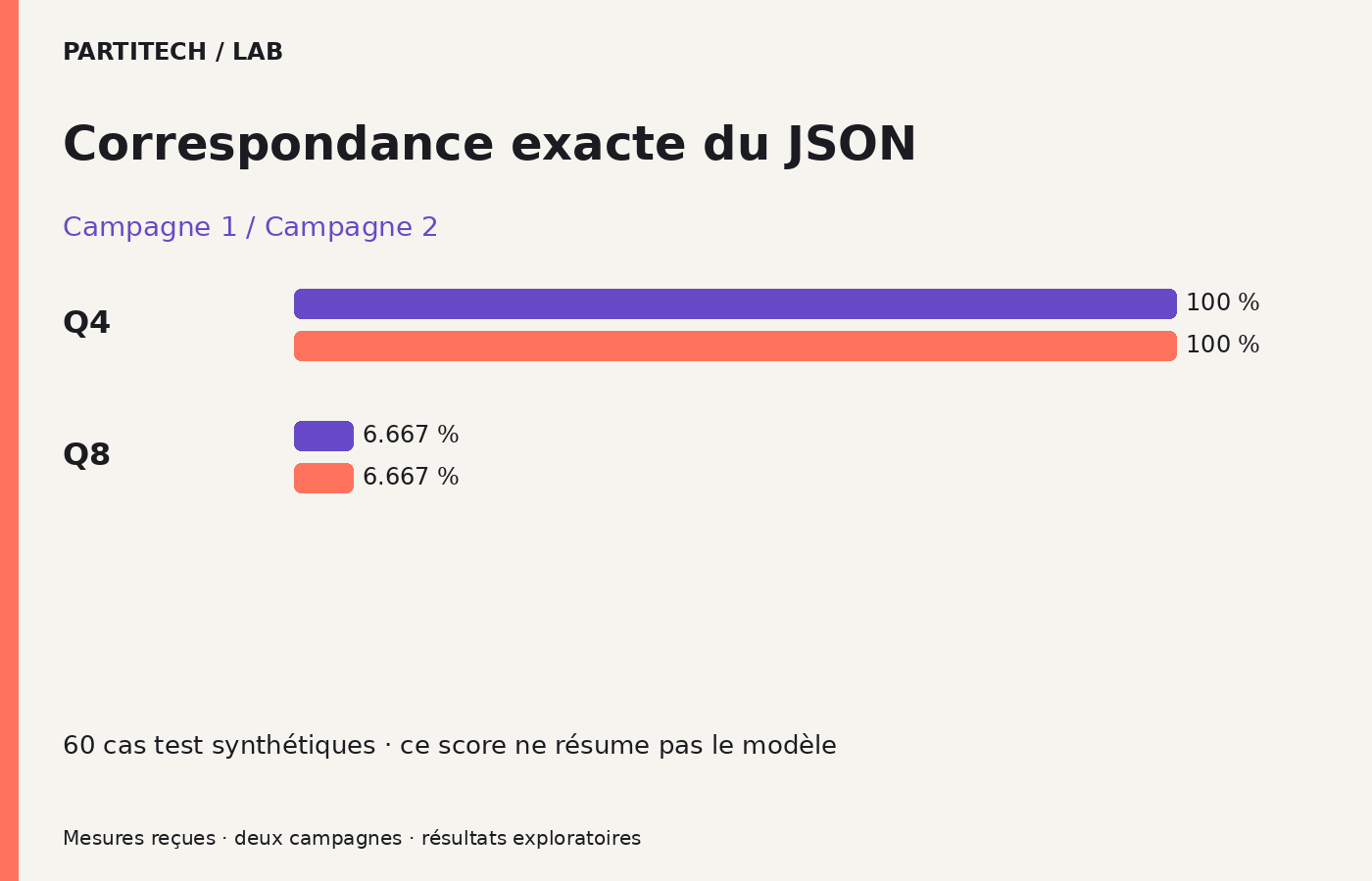
The visual's mention of "60 synthetic test cases" belongs to the original document. It does not replace the 80-case scope specified for each mode.
Scope and documented rerun
The observations concern synthetic data, a single host, and a frozen software stack. Re-running the experiment depends on the local Lab foundation, the llama.cpp image, and the locked models.
This resembles an integration test for which you keep the code, datasets, and service versions. Reading its results again is not the same as running it again; running it with different dependencies does not necessarily reproduce the same experiment.
The project also contains metric functions and tests for their inputs. Here is the provided excerpt, likewise reformatted without changing its logic.
Frozen source: poc/metrics.py, lines 30–44. SHA-256 of the recorded source file: 9d39a8d113cc112f5ece7ecbf6454f0cbe46ceddd847c4af25789ead12171899.
def valid_query(q):
    if not isinstance(q, str) or not q.strip() or len(q) > 2048:
        raise ValueError('invalid query')
    return q


def unit():
    assert (
        distance('chat', 'chats') == 1
        and distance([], ['x']) == 1
        and distance('abc', 'adc') == 1
    )
    assert normalize('ÉTÉ, bonjour!') == 'été bonjour'
    assert rank_metrics([2, 1], [1]) == {
        'recall5': 1.0,
        'mrr10': .5,
        'ndcg10': 1 / math.log2(3),
    }
    assert rank_metrics([2], []) == {
        'recall5': 0,
        'mrr10': 0,
        'ndcg10': 0,
    }
    assert bm25(
        [{'id': 0, 'text': 'chat'}, {'id': 1, 'text': 'chien'}],
        'chat',
    )[0][0] == 0
    assert bm25([], 'x') == [] and rrf([(1, 1)], [(2, 1)])[0][1] == 1 / 61

    for x in ['', None, {}, 42, 'x' * 2049]:
        try:
            valid_query(x)
        except ValueError:
            pass
        else:
            raise AssertionError('query guard')
Reading valid_query() as form validation
This function requires a string, rejects an empty or whitespace-only string, and imposes a maximum length of 2,048 characters. When any of these conditions fails, it raises ValueError('invalid query').
One detail deserves attention: q.strip() is used only for the check. The function returns q, not q.strip(). It therefore does not remove spaces from the value returned to the caller.
In unit(), the loop tries several forbidden inputs: an empty string, None, a dictionary, a number, and a 2,049-character string. If one passes without an error, the test fails with AssertionError('query guard'). This is the same logic as a backend test checking that a missing or overly long field is rejected.
Why are search and ranking tests included too?
The other assertions check distance, normalization, ranking, and search functions in the metrics module. For example, the normalize() test expects ÉTÉ, bonjour! to become été bonjour: in this example, case and punctuation change, but accents remain.
The names rank_metrics, bm25, and rrf appear in the excerpt. Their presence does not mean that the Q4/Q8 score combines all these tests, nor that the experiment sets up a search engine. This block checks utilities; by itself, it does not show the full strict-equality calculation.
The key idea is simple: the program that performs the measurement must itself be tested. But passing its unit tests demonstrates neither the model's overall quality nor the representativeness of the dataset.
Local assets and recorded versions
To rerun this experiment, Python code is not enough. You also need the weight files, Docker images, and Lab foundation at the documented versions. These are the local assets mentioned in the folder: the items needed for execution that are already on the workstation.
The environment lock records, among other things, the driver and the llama.cpp image. The model lock identifies Qwen2.5 7B and the Q4_K_M and Q8_0 GGUF files by their hashes. The package downloads nothing automatically.
You can compare this principle to a composer.lock file or a JavaScript dependency lock: the goal is to recover a precise configuration, not merely components carrying the same name.
A SHA-256 hash is a value calculated from a file's contents. It lets you compare the file at hand with the expected one instead of trusting its name. The Python documentation for hashlib presents this family of functions. Here, hashes identify the experiment's assets; they do not by themselves prove their quality or that of the results.
How the launcher prepares the experiment
The README associates this topic with a labctl command, to be run from the already installed Lab. labctl is this environment's launcher: it is not a command supplied by Python or Docker.
According to the recorded procedure, it adapts paths in the Docker Compose template, checks asset hashes, then starts the Python program in the container. The template is the starting configuration; adaptation lets it receive the expected locations on the relevant workstation.
The paths need some attention. /poc and /assets are paths inside the container. Paths beginning with /llm, visible in the captures, belong to the original workstation. Copying them exactly to another machine does not guarantee that they point to the right files there.
The exact launch is retained in the reproduction section together with its prerequisites. Describing this procedure explains how to rerun the experiment; it does not mean a new run was performed while preparing the article.
Measurement safeguards visible in the frozen code
Let us return to quant(). Each step answers a question very similar to those you would ask when testing an API.
Is the service ready to receive the request?
ready('http://server:8080', '/health') waits for the local service. The returned duration is recorded in a load event with the ready_seconds field.
The name load should not make us forget what the excerpt actually shows: waiting for availability. Without reading ready()'s implementation, we cannot treat this value as the GPU weight-loading time alone.
Is the first request distinguished from the measurement loop?
Before the loop, the program calls llm() with the first dataset query. This is the warm-up request specified by the protocol. It prepares the path before calls recorded as samples.
This line is not accompanied by emit('sample', ...) in the excerpt. The loop then takes every query again, including the first, and emits a sample event for each one. You must therefore distinguish the number of cases in the dataset from the total number of calls made, which also includes warm-up and the overlong-input test.
Can an answer be linked back to its question?
In the loop, q['query'] provides the request and q['id'] its identifier. The **r notation passes result fields to emit().
The identifier matters: it lets you find which output belongs to which case, then examine disagreements. Without this link, a global score alone could not identify the references missing the REF- prefix.
Is an intentionally excessive request rejected?
The program then sends 'mot ' * 10000, that is, the string mot repeated 10,000 times. It expects an HTTP exception with code 400 or 413. If this call is accepted, it raises AssertionError('oversize accepted').
This is a negative test: it deliberately sends an input the path must reject. A return without an error is therefore not a test success but a failure.
Keep two reading limits in mind. First, 10,000 repetitions do not necessarily mean 10,000 tokens. Second, the excerpt checks these two HTTP codes; by itself it does not prove handling of every input size or every possible error.
The 2,048-character guard in valid_query() and this context test are not interchangeable either. The first checks a text input at the level of a Python function. The second asks the inference path to reject an excessive input. Since the body of llm() is not reproduced, we must not invent how every check is chained internally.
Finally, emit('complete', ...) is reached only if the path gets as far as that instruction. Finding this event is useful, but you must also check the number and identifiers of samples: an end marker does not replace data verification.
Checking, exporting, and removing work traces
The exported evidence includes metrics from both campaigns, validation checks, and capture logs referenced in the folder. Its role is to allow observations to be reviewed without having to publish content or immediately run the model again.
To inspect them, start with a result and trace back to its request, its recorded answer, and then the rule that produced its score. Then check that every stated case is covered, errors are retained, and protocol tolerances are respected. This is notably the stage at which the link between the 80- and 60-case scopes must be clarified.
The package described here performs no CMS, media, or social-network operation. Work files and local assets remain managed in the Lab environment. Exporting and cleaning them up must not be confused with publishing this article.
A score calculated outside the model's answer
Imagine that your endpoint could decide for itself whether its integration test passed. That would not be an independent check. The same precaution applies here: the model produces an answer; another piece of code compares it with what is expected.
The metrics module specifies pure scorers, used offline by the recorder, the tool that records and processes results. In this context, "pure" means that score calculation depends on its inputs, without asking the model to evaluate itself. The folder therefore refers to a deterministic review, not a human opinion or an LLM grade.
This separation makes it possible to recalculate a score from an answer already captured. It does not make the model's generation automatically deterministic. Recalculating on the same outputs and obtaining new outputs from the model are two different operations.
The module contains a normalization function and input validations, but their presence is not enough to establish every transformation applied to this topic's strict score. The documented point remains this: omitting REF- fails this equality even when quantities and categories are retained.
Short exercise: would your application accept the answer?
Return to the two illustrative JSON objects presented above. Before rereading the explanation, ask yourself what you would accept for a demonstration screen, then for a product lookup by exact identifier.
Let us add a third imaginary situation: the reference is indeed REF-042, but the quantity changes from 3 to 30. The JSON can still be decoded without difficulty. Yet the answer is no longer correct for the described need.
The exercise is to explain separately what concerns syntax, reference format, and business value. It produces no new benchmark result.
One might suggest a rule that automatically adds REF- to incomplete references. That would be a processing change, not a simple rereading of current results. Before using it, you would need to define the cases where this correction is allowed, check that it introduces no ambiguity, and test it separately. The scores published here do not measure that variant.
Reading latency and throughput together
For your application, a duration answers the question "how long does this call take?" Throughput instead answers "how quickly is text processed or produced?" This information is complementary; it is not interchangeable.
Thus, 93 tokens per second does not mean 93 requests per second. To move from one to the other, you would need to know, among other things, the length of requests and answers as well as how calls are organized. The published measurements do not describe this serving capacity under load.
Q4 shows lower latencies and higher throughput than Q8 here. That describes these cases, on this workstation, with this stack. The two campaigns cover neither simultaneous users, real non-synthetic prompts, hardware changes, nor energy consumption.
VRAM is another matter. A 1 Hz sample provides only one observation per second: a shorter peak can occur between samples. The summary provides no memory-use values with which to quantify a Q4/Q8 gain here. We therefore infer neither a precise VRAM saving nor a validated hardware minimum.
To read the table without making it say more, always keep the variant, case set, output contract, and measurement method together. The number alone is not enough to select a configuration for another product.
Sources and provenance limitation
Where do the results come from?
The original document states that the editorial team cross-checked the report, metrics, protocol, locks, and final archive validation. It also reports that a control recalculation recovers the captured values. The results presented here are those of this folder, not of a new campaign run for this educational version.
One limitation must remain visible: the sources used during captures correspond to distinct historical versions of the installed Lab foundation. This difference must be retained in the audit folder. It does not, by itself, invalidate the reported internal consistency between observations; however, it prevents assuming that the current foundation automatically reproduces the historical code.
This is comparable to the difference between the commit that produced a CI result and the branch currently open in your editor. To understand an older result, you retain the identity of the code that produced it.
Two notes whose connection to the topic remains to be clarified
The original record also includes the note "Synthetic data except FLEURS" and a note identified as 010: compared context capacities, deterministic prompts below the limit, and generation of 64 tokens.
The Q4/Q8 topic is identified as 006. The supplied material does not explain how these two notes relate to its measurements. They are retained as provenance indications, but we infer neither that FLEURS is part of the Q4/Q8 cases nor that generations in this comparison have a 64-token limit. These points must be established in the relevant protocol, not filled in by assumption.
What are the supplementary references for?
Links to Qwen, GGUF, llama.cpp, Python, and Docker documentation explain concepts. They do not replace the experiment's locked versions and add no GPU validation. Current documentation may show other models or commands: it does not authorize substituting them for the measured path.
Traceability of this experiment
This section brings together the elements needed to identify the campaign and understand the conditions for rerunning it. You can read it as a test data sheet: what was it run with, when, and from which files?
The model and its files
The two variants come from Qwen/Qwen2.5-7B-Instruct-GGUF, at revision:
bb5d59e06d9551d752d08b292a50eb208b07ab1f
The licenses declared in the folder are Apache-2.0 for q4 and apache-2.0 for q8. Individual file hashes are retained in locks/models.lock.json.
This information identifies the tested assets. It does not identify a currently recommended version. The repository at that exact revision lets you distinguish these files from those in a branch that may have changed.
Recorded hardware and environment
This topic's computation uses one RTX 3090. The workstation's two GPUs are reserved during measurements: this does not mean computation is distributed across two cards.
The recorded driver is 580.95.05. The running client image is identified by:
sha256:545518febcd04dce9c9d8b1168af1ce518508901adb517489028ccb5b456ecc2
This client-image hash must not be renamed as the llama.cpp server hash. The folder records environment elements separately.
The Linux distribution and exact version are not recorded in this lock. This information therefore does not demonstrate compatibility with every Linux installation.
The two runs of September 11, 2026
First campaign. run_id: 20260911t123640-73f55072a554. Recorded start: 2026-09-11T12:36:40.823741+00:00. Captured duration: 63.48 s.
Second campaign. run_id: 20260911t123744-fc0c359a445d. Recorded start: 2026-09-11T12:37:44.604541+00:00. Captured duration: 63.99 s.
The +00:00 suffix indicates that these timestamps are in UTC. The durations concern captured commands, not total installation, download, or intervention time.
The delivery is identified as r1. The recorded code hash is:
e94fd5ca24d24d216757e79747f1c555bd142b3a81f39a0c81346a07d3eebfea
The second campaign starts again from a fresh workspace and fresh application volumes. Verified immutable assets are reused: "clean run" therefore does not mean "downloading every file from scratch."
Both campaigns remain observations on the declared workstation. The folder indicates that calculations were checked from received outputs; no training or GPU inference was rerun on the editorial workstation.
Before launching: have the Lab and assets available
The starting point is the Lab supplied with the POC, the experimental demonstration project, already installed on the GPU workstation. It includes labctl, lab/, batchkit/, scripts/, and the locks.
The ZIP contains the program and evidence, but not the Docker images or model weights. No public POC download URL was created for this delivery. The complete code is in the work kit; the excerpts on this page alone cannot reconstruct a validated installation.
You need Docker Compose and NVIDIA GPU access, then must obtain the assets at the specified revisions and hashes. The Compose template uses workstation-specific paths and pull_policy: never: images must already be present. According to the official Docker Compose reference, this policy prevents automatic image downloading and fails if the image is missing locally.
Weights and data are mounted read-only. Do not replace a revision with main, a specific image with latest, or a verified file with different weights simply to work around a missing asset: you would change the experiment.
Running the documented command
Go to the installed Lab directory. The following command is the one extracted from the README; the launcher prepares paths and the Compose project, then runs the program in the container.
Frozen source: poc/README.md, line 4. SHA-256 of the recorded source file: ad09840e896cada8ad36cfc3bc888a6aca9492a857591026d9c59964795324ee.
./labctl run --machine gpu --batch 2026-09-11 --topic gguf-q4-q8-mesures
The options identify the GPU machine, the 2026-09-11 batch, and the gguf-q4-q8-mesures topic. This date identifies the work batch; it is not future scheduling.
After execution, retain outputs, errors, and test files. Check samples, their coverage, and both campaigns' tolerances from the recorded elements rather than limiting yourself to the absence of an error in the terminal.
An already PACKAGED state does not necessarily trigger a new experiment during a resume. To find out whether you actually replayed the computation, locate the run and its run_id. The two documented clean reruns are those identified above.
Any change to code, data, model, or protocol requires a new revision and new captures. Old scores must not be reassigned to that variant.
In case of an error, then cleanup
A missing image, nonexistent mount, or exceeded timeout signals a prerequisite to resolve. Stop the path and identify what is missing. Quietly changing the inference engine or parameters to obtain a successful run would not reproduce the documented test.
Cleanup for this path belongs to the launcher and its Compose project. The supplied Makefile provides no standalone clean target; no global purge command is therefore proposed. Keep private archives and shared weights, which may serve other experiments.
What we learned
Q4 achieves a better strict score and better latency and throughput measurements than Q8 here. This result applies to two campaigns, one model at a precise revision, synthetic data, and a given output contract.
The most useful point for a developer lies in the answers: a correct quantity does not necessarily compensate for an incomplete reference. You must know what your application expects before deciding what a "good score" means.
We also distinguished three activities: reviewing recorded answers, recalculating their scores, and replaying the model. They are complementary, but they are not the same validation.
To apply this method to another project, start by defining your output contract and test cases. Examine concrete errors, then measure performance under the conditions that matter to you. The right choice is not the one whose name sounds most reassuring: it is the one whose behavior you have verified for your use.