





You are developing a dashboard that shows the load forecast for tomorrow. Only one value appears: “50 kW at 2 p.m.” It is a start, but a question immediately follows: should you prepare for a value close to 50, or for a much larger variation?
A central curve does not answer that question. We will therefore learn to produce three estimates for each hour: a low, a median, and a high one. The aim is not to make the future certain, but to give uncertainty a measurable form.
The starting case is an illustration. In the experiment, we use simulated series only: no real meter and no energy decision depends on our forecasts.
Download the tutorial archive.
What we build
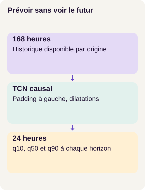
The program simulates twelve hourly series, then trains a network to use the previous 168 hours, or seven days, to forecast the next 24 hours. For every future hour, it produces q10, q50, and q90.
You can picture its input as the result of a query on a measurement table: one site, ordered hours, and the values already available. Its output is a 24-row table, with three estimates per row. This comparison helps explain the data contract; the project provides neither a business API nor a connection to a production database.
We compare three methods: a seasonal reference called a baseline, a network with independent outputs, and a network with ordered outputs. Both networks use a causal TCN, whose operation we will explain. The difference between their “heads” concerns how the three final values are constructed.
By the end, you will be able to follow the path from data to predictions, calculate quantile loss, check that time order is respected, and interpret the results. The numbers remain simulated kW: this tutorial is not an operational energy forecast.
Concepts: what quantiles guarantee, and what they do not
Three thresholds rather than one value and an arbitrary margin
A quantile is a threshold associated with a proportion. Here, we seek conditional quantiles: they depend on the history available and apply to a particular future hour.
Consider an educational example, separate from the model’s outputs:
| Estimate | Illustrative value | What we aim to estimate |
|---|---|---|
q10 |
42 kW | A threshold below which approximately 10% of values would fall under the conditions considered. |
q50 |
50 kW | The median: a value that divides the distribution into two halves. |
q90 |
63 kW | A threshold below which approximately 90% of values would fall under the conditions considered. |
The band runs from 42 to 63 kW. Its width is therefore 63 − 42 = 21 kW. It targets coverage of 90% − 10% = 80%.
Notice that the median is not necessarily in the middle of the band: here, it is 8 kW from the lower bound and 13 kW from the upper bound. We did not impose a symmetric margin such as “central value ± 5.”
q90 does not mean “a prediction that is 90% accurate.” This number denotes the quantile level sought, not a confidence score assigned to the answer. Likewise, q50 denotes the median, not necessarily the mean.
The network estimates these thresholds for the future. It does not simply sort the 168 past values and extract three positions from them. The official scikit-learn quantile regression example illustrates this distinction between central prediction, quantiles, and observed coverage.
How can a quantile be learned from a single real value?
For a given hour, we do not have one hundred possible futures: we observe only one value. How can we teach three quantiles to the network?
We present it with many histories, each accompanied by the values that actually followed. A loss function assigns a cost to errors. By accumulating these costs over the examples, training adjusts the network parameters.
To learn a median, an upward error and a downward error of the same magnitude are penalized in the same way. To learn a high quantile, we penalize an estimate that is too low more heavily. This is the role of pinball loss, or quantile loss.
Let y be the observed value, q the predicted value, and τ—the Greek letter “tau”—the quantile level. In our case, τ is 0.1, 0.5, or 0.9.
The formula is:
error = y − q
loss = max(τ × error, (τ − 1) × error)
There is no need to memorize this notation before understanding it. For a target of 50, here are the costs of two hypothetical predictions:
| Prediction | Error y − q |
Cost for q10 |
Cost for q50 |
Cost for q90 |
|---|---|---|---|---|
| 48: too low by 2 | +2 | 0.2 | 1.0 | 1.8 |
| 52: too high by 2 | −2 | 1.8 | 1.0 | 0.2 |
For q90, underestimating by 2 therefore costs 0.9 × 2 = 1.8. Overestimating by 2 costs only 0.1 × 2 = 0.2. For q10, it is the opposite. The penalties remain positive or zero; what changes is their weight according to the direction of the error.
Why would the network not keep raising q90 indefinitely? Because overestimating costs less, but it does not cost zero. The loss seeks a trade-off over all examples, not a bound that encompasses everything at any price. The pinball loss documentation uses the same calculation convention.
A TCN: filters that move through time
TCN stands for Temporal Convolutional Network. A convolution combines several neighbouring values with learned coefficients. You can compare it to a moving average, with one essential difference: the network learns the coefficients and combines several operations instead of receiving a hand-defined averaging rule.
A causal temporal filter works only with the current position and earlier positions. In a three-value example, the output at time 10 can read times 8, 9, and 10, but not time 11.
Dilation spaces out the positions that are read. Still using this three-value example:
Dilatation 1, sortie au temps 10 : lecture des temps 8, 9 et 10.
Dilatation 2, sortie au temps 10 : lecture des temps 6, 8 et 10.
Dilatation 4, sortie au temps 10 : lecture des temps 2, 6 et 10.
These indices illustrate the mechanism, not the exact configuration of the delivered network. By stacking layers, we widen the receptive field, that is, all positions that may influence an output. Providing 168 hours to the program and demonstrating that its architecture can use all of them are two separate checks.
The principle of dilated causal convolutions is described in the study by Bai, Kolter, and Koltun. Here, “causal” means respecting the temporal order of information. It does not mean that the model has identified the physical causes of a change in load.
Padding: completing an edge without reading beyond it
At the beginning of a sequence, some positions required by a filter do not exist. Padding consists of completing that edge with fill values. The tutorial’s TCN uses left padding, on the past side, to preserve causal behaviour.
A centred convolution can, by contrast, use a position to the right of the one it computes. At time 9, a filter centred on three positions would read 8, 9, and 10: value 10 could then change an output assigned to time 9. The final exercise makes this difference observable.
This internal control does not replace a check of the data. A causal network can still receive a poorly constructed history containing information unavailable at the time of forecasting. We will therefore also check the window split and preprocessing calculation.
Two heads: estimate freely or impose an order
The head is the final part of the network that turns what it has calculated into output values.
With the independent head, the three outputs are not constrained to follow an order. For example, the network could propose q10 = 52, q50 = 50, and q90 = 49. That would be a crossing: the supposed lower bound would exceed the upper bound. “Independent” here describes the absence of that constraint; it does not mean that hours or series are statistically independent.
The ordered head starts from q10, then adds increments obtained with softplus. Its principle reads as follows; the letters a, b, and c are teaching notation for three raw outputs:
q10 = a
q50 = q10 + softplus(b)
q90 = q50 + softplus(c)
In its usual form, softplus(x) = log(1 + exp(x)). It turns a value into a positive increment while remaining suitable for gradient computation. The PyTorch documentation for softplus details this operation and its numerical implementation.
For example, softplus(0) = log(2) ≈ 0.6931. With a = 48, b = 0, and c = 0, the three outputs become approximately 48, 48.6931, and 49.3863. This example explains the construction; it is not a prediction captured in the experiment.
For finite outputs, this construction enforces q10 ≤ q50 ≤ q90. It does not require the load to increase over the 24 hours, q10 itself to be positive, or the band to contain the correct proportion of observations.
Think of form validation that enforces “start date ≤ end date.” It checks a consistent order; it does not prove that the dates match the actual appointment. An ordered band is not automatically a well-calibrated band.
Docker and GPU prerequisites
You should be comfortable with Python functions, arrays, a terminal, and Docker basics. Learning concepts are introduced in the track; you do not need to already know TCNs.
The track expects Linux x86_64, Docker Compose, NVIDIA Container Toolkit, and a 24 GiB RTX 3090, as well as 16 GiB of available RAM and 16 GiB of disk space, excluding shared Docker layers. It uses one card; owning two GPUs does not mean you must use both for this exercise.
The GPU is the graphics processor used for the network’s computations. Here CUDA lets PyTorch use it. The environment check initialises CUDA from inside the container and runs a calculation: seeing a card on the host is not enough. This check must succeed before training. The Docker documentation on GPU access and the NVIDIA Container Toolkit guide describe this integration.
To select the card, export GPU_DEVICE=0 or a card UUID before the commands. The UUID is its identifier; it is another way to select it instead of its index. Keep the supplied GPU track to reproduce the results: no equivalent CPU result is presented here.
GPU computation runs without network access. The containers use a read-only filesystem, no-new-privileges, dropped Linux capabilities and CPU, RAM and PID limits. In web-development terms, this limits what a process can do and consume; it does not certify its predictions.
A checkpoint is a saved state that lets you reload or resume a computation. Do not load a Torch checkpoint from an untrusted source.
Data: separate time before training
A small world whose rules we know
The simulator produces 12 series of 180 days, or 180 × 24 = 4,320 hourly values per site. Each series combines a baseline level, a daily cycle, a weekly cycle, random fluctuations, and a few one-off events.
The cycles give the network regularities to learn. The fluctuations prevent the future from being reduced to a perfectly deterministic repetition. We know the recipe for the data, which makes checks easier; that does not make them representative of real sites.
The split is chronological, with days numbered starting at zero:
| Data split | Days | Role |
|---|---|---|
Training, or train |
0–119 | Learn the network parameters and fit the scaler. |
| Validation | 120–149 | Examine the model over a later period, separate from training. |
| Test | 150–179 | Measure results over the final held-out period. |
A scaler transforms the scale of numbers before the model uses them. When such a transformation learns statistics, those statistics must come from train only. Using all 180 days to calculate them would already convey information about future periods, even without directly providing their targets to the network. This risk of leakage through preprocessing is explained in the scikit-learn documentation on data leakage.
The project rule is therefore: fit on train, then keep this transformation for the other periods. The exact scaler type remains the one in the delivered code; you do not need to replace it with different normalization to follow the tutorial.
Reading the simulator
The following excerpt creates the series and keeps the parameters that produced them. np refers to NumPy and TEST_END to the hourly bound defined in the project. These are excerpts from the complete program: the Docker commands below run the whole thing, with its imports and configuration.
def simulate(seed=17):
    rng = np.random.default_rng(seed)
    t = np.arange(TEST_END)
    series = []
    parameters = []
    for site in range(12):
        baseline = 35 + 2 * site
        daily = 5 + 0.3 * site
        weekly = 3 + 0.1 * site
        phase = 0.17 * site
        noise = 1.2 + 0.05 * site
        value = (
            baseline
            + daily * np.sin(2 * np.pi * t / 24 + phase)
            + weekly * np.cos(2 * np.pi * t / 168)
            + rng.normal(0, noise, len(t))
        )
        events = []
        for day in (25 + site, 75 + site, 125 + site, 155 + site):
            start = day * 24 + 8
            amplitude = 4 + site / 3
            value[start : start + 8] += amplitude
            events.append({"start": start, "duration": 8, "amplitude": amplitude})
        series.append(value)
        parameters.append(
            {
                "site": site,
                "baseline": baseline,
                "daily_amplitude": daily,
                "weekly_amplitude": weekly,
                "phase": phase,
                "noise_std": noise,
                "events": events,
            }
        )
    return np.asarray(series, dtype="float32"), parameters
What just happened?
np.random.default_rng(seed) initializes the pseudorandom generator. The default seed is 17. In an unchanged environment, repeating the same operations with this seed reproduces the same draws.
The loop visits sites 0 through 11. baseline = 35 + 2 * site gives each one a different background level. Watch the vocabulary: this baseline variable is the signal’s base level, not the seasonal reference model compared later.
The terms sin(... / 24 ...) and cos(... / 168 ...) add daily and weekly oscillations. The daily and weekly amplitudes set their importance, while phase shifts the daily cycle. rng.normal(0, noise, len(t)) adds zero-centered Gaussian noise; noise sets its standard deviation and thus the magnitude of its fluctuations.
The second loop adds four eight-hour events per site. For site 0, for example, the event on day 25 starts at index 25 × 24 + 8 = 608. The slice 608:616 increases eight values by 4. This is a reading of the simulator formula, not the forecast learned by the network.
Finally, the function returns a float32 array and the parameters list, which documents the generation. float32 indicates that numbers are stored as 32-bit floating-point values.
Scope of the excerpt: simulate() creates the values and their parameters; it does not contain window construction or the choice of origins. Those operations belong to the full preparation. Knowing the events in the simulator does not authorize providing them to the model as future information either.
An origin: the point in time from which we forecast
A forecast origin is the starting point of a forecast. To interpret the indices, let us call the first hour to predict T. Under this explanatory convention:
Historique visible : T − 168, ..., T − 1   → 168 valeurs déjà connues.
Cibles à prévoir   : T, ..., T + 23       → 24 valeurs futures.
During training, these targets are known to the program and are used to calculate the error. They must not be mixed with the history supplied as input. It is the same principle as a test set: the expected answer is used to correct the result, not to fill in the data of the function being tested.
Training windows advance by one hour. Their targets must remain entirely within train. Validation and test use one origin per day and per site:
12 sites × 30 days = 360 origins per split
360 origins × 24 hours = 8,640 hourly targets per split
That represents 8,640 values to check, not 8,640 days. Each value receives three estimates, or 8,640 × 3 = 25,920 elementary contributions to quantile loss.
Crossing a boundary with history is not necessarily leakage
Take the first validation origin, at the start of day 120. Days 113 to 119 form a seven-day history that is already available. The fact that these values belong to train is not a problem: they are in the past of this forecast.
By contrast, a training window whose first target is the last hour of day 119 would spill into day 120 for its other targets. It would mix training and validation and must be excluded.
The same logic applies to the test. At the start of day 150, days 143 to 149 are already known. Later, observations from the start of the test period can serve as history for a later origin, if they are actually available on that date. This does not mean retraining the network or refitting the scaler on the test.
Evaluation therefore replays successive forecasts. It does not predict the thirty test days all at once from their first morning.
The core code: quantile loss
Understanding dimensions before operations
Here, a tensor is an array of numbers with several dimensions. In a batch of B examples, where B is the number of windows processed together, we have:
prediction : B × 24 × 3   → un triplet q10, q50, q90 pour chaque heure.
target     : B × 24       → une seule valeur observée pour chaque heure.
For a single example, the network therefore proposes 72 numbers and we have 24 reference values. The three predictions for one hour are compared with the same target, with three different penalties.
def pinball_loss(prediction, target):
    tau = torch.tensor(
        [0.1, 0.5, 0.9], device=prediction.device, dtype=prediction.dtype
    )
    error = target[..., None] - prediction
    return torch.maximum(tau * error, (tau - 1) * error).mean()


def check_loss(config):
    p = torch.zeros(1, 1, 3)
    positive = pinball_loss(p, torch.ones(1, 1))
    negative = pinball_loss(p, -torch.ones(1, 1))
    assert torch.allclose(positive, torch.tensor(0.5)) and torch.allclose(
        negative, torch.tensor(0.5)
    )
    return {
        "e_plus_1": [0.1, 0.5, 0.9],
        "e_minus_1": [0.9, 0.5, 0.1],
        "mean_positive": float(positive),
        "mean_negative": float(negative),
    }
Reading the three operations in pinball_loss()
tau contains the levels [0.1, 0.5, 0.9], in the same order as the three outputs. device and dtype give it the same computation location and numeric type as prediction.
target[..., None] adds a dimension of size 1 at the end of the array: B × 24 becomes B × 24 × 1. PyTorch can then compare each target with its three corresponding predictions. This implicit expansion of compatible dimensions is called broadcasting; the PyTorch documentation describes its rules.
Finally, torch.maximum(...) chooses the appropriate cost for each error. .mean() averages all these costs: over the examples in the batch, the 24 hours, and the three quantiles. The result is a scalar, that is, a single number.
The function calculates the loss, but does not itself modify the parameters. During training, gradients indicate how a change in parameters would affect that loss, then the optimizer applies the updates. During evaluation, the same loss can be calculated without training anything.
A calculation you can repeat by hand
Take a fictional hour with y = 50 and predictions q10 = 47, q50 = 51, q90 = 55.
The low quantile underestimates by 3: its cost is 0.1 × 3 = 0.3. The median overestimates by 1: its cost is 0.5 × 1 = 0.5. The high quantile overestimates by 5: its cost is 0.1 × 5 = 0.5.
The mean loss for this hour is therefore:
(0.3 + 0.5 + 0.5) / 3 = 0.4333…
The actual value is indeed within the [47, 55] band, but the loss is not zero. This is not a contradiction: being covered and having a good quantile score are not the same check.
At τ = 0.5, pinball loss equals half the absolute error. This identity concerns the median component, not the mean of the three quantiles. The mean_pinball_loss reference lets you recover this property.
The loss has the unit of the numbers supplied to it. The measurements published below are expressed in simulated kW; a loss calculated on a transformed scale should not be compared directly with those values without taking the scaler into account.
What check_loss() checks, and what it does not check
The check constructs three zero predictions, then a +1 target and a −1 target. The expected contributions are respectively [0.1; 0.5; 0.9] and [0.9; 0.5; 0.1]. Their mean is 0.5 in both cases.
The assertion does check these two means, with torch.allclose, which compares values using a numerical tolerance. By contrast, the e_plus_1 and e_minus_1 lists returned by the function are hard-coded, not recalculated from the intermediate contributions.
A point to watch: this average is not enough to detect a sign reversal. With these three symmetric levels and identical predictions, replacing
target − predictionwithprediction − targetwould swap the contributions of the low and high quantiles without changing the average of0,5. The displayed formula does use the correct direction; the scope of this assertion must be distinguished from that of a per-quantile check.
To strengthen this check in a separate experiment, we would need to compare the contributions of each level or add different predictions according to the quantile. The reference code above remains unchanged. This observation does not determine the content of the project’s other tests.
Install and check the environment
Extract the archive, then place your terminal at its root, where the scripts and Compose configuration are located. All the commands that follow run from that same directory.
This project has no pretrained weights to download: here, acquire validates a manifest with no weights. The series will be made by prepare, and the network will be trained on those data. The role of this step differs from acquiring a large language model.
sh scripts/setup.sh
docker compose config --quiet
docker compose build acquire gpu
docker compose run --rm acquire python scripts/acquire.py --config configs/minimum.yaml
docker compose run --rm gpu python scripts/check_environment.py --config configs/minimum.yaml
docker compose run --rm gpu python -m pytest -q
Read this sequence as preparing a development environment. setup.sh prepares the project; config --quiet checks the Compose configuration; build acquire gpu builds the images for the two services. Next come manifest validation, the CUDA check computation in the container, and the test suite with pytest.
Expected observation: every command must finish without an error. The environment check must succeed before training. A successful test suite checks the program on its intended cases; it has not yet measured forecast quality on the test set.
Keep the archive’s versions and settings for reproduction. The references at the end of the article are there to understand the mechanisms, not to replace the project dependencies with their latest versions.
Prepare, compare, and train
We can now create the data, establish the seasonal reference, inspect the network, check the loss, and train both heads. The sequence also contains an intentional stop, a resumption, and a comparison of states before evaluation.
The results published below come from the validated reader reproduction of this r1 workflow.
docker compose run --rm gpu python -m quantile_forecast.cli prepare --config configs/minimum.yaml
docker compose run --rm gpu python -m quantile_forecast.cli baseline --config configs/minimum.yaml
docker compose run --rm gpu python -m quantile_forecast.cli inspect-model --config configs/minimum.yaml
docker compose run --rm gpu python -m quantile_forecast.cli check-loss --config configs/minimum.yaml
docker compose run --rm gpu python -m quantile_forecast.cli train --config configs/minimum.yaml
docker compose run --rm gpu python -m quantile_forecast.cli train --config configs/minimum.yaml --variant independent
docker compose run --rm gpu python -m quantile_forecast.cli train --config configs/minimum.yaml --stop-after 1000 --run-name interrupted
docker compose run --rm gpu python -m quantile_forecast.cli train --config configs/minimum.yaml --resume artifacts/checkpoints/interrupted/state.pt --run-name resumed
docker compose run --rm gpu python -m quantile_forecast.cli compare-resume --config configs/minimum.yaml
docker compose run --rm gpu python -m quantile_forecast.cli evaluate --config configs/minimum.yaml
Prepare a reference before asking more of the network
prepare prepares the series and windows according to the described time rules. baseline establishes the seasonal reference: a comparison point that exploits the repetition of patterns over time.
The purpose of a baseline is not to create an opponent that is easy to beat. It lets us ask a useful question: what does the network add compared with a reference method? The details of this baseline remain those in the archive; the excerpts in this article do not give its complete formula.
inspect-model comes before training and lets you check the network. check-loss performs the numerical check we have just read. Review their results before starting the most costly part of the workflow.
Compare two output constructions
The workflow’s train command trains the ordered head; --variant independent starts the independent variant. Their comparison covers, among other things, quantile error, the median, coverage, width, and crossings.
Do not replace one head with a simple sorting of results before evaluation. Sorting afterward would create another processing step, whose outputs would have to be retained and whose effects measured separately.
Resume: continue a state, not restart a run
The command with --stop-after 1000 --run-name interrupted deliberately stops training at step 1,000. A step is one stage of training; this number denotes neither one thousand forecast hours nor one thousand days of data.
The next command reloads artifacts/checkpoints/interrupted/state.pt and continues under the name resumed. compare-resume then compares the resumption with the reference workflow.
You can compare this operation to resumable queue processing: finding the last file written is not enough if the state needed to continue at exactly the same point has been lost. The project’s resume test makes this continuity verifiable instead of assuming it.
Finally, evaluate produces the measurements for the compared methods. A zero maximum error during resumption and good forecasting accuracy are two distinct results: one concerns computational continuity, the other the quality of the outputs.
Measurements before results
Each result aggregates 360 origins and 8,640 hourly targets. Before comparing figures, let us establish the meaning of each measurement.
Pinball: the quality of the three thresholds
Mean pinball loss applies the preceding calculation to the three quantiles. Here it is expressed in simulated kW. Lower is better, for the same population, the same quantiles, and the same unit convention. It is not a percentage of exact forecasts.
MAE: the median’s error only
MAE, short for Mean Absolute Error, is the average of the absolute differences. In this tutorial, it concerns q50:
MAE = average of |observed value − q50|
A median of 50 against an observation of 53 contributes 3 kW. The lower and upper bounds do not participate in this calculation. “Median MAE” therefore means the average of the q50 errors, not the median of all errors.
Coverage: how many values fall inside the band?
A target is covered when q10 ≤ y ≤ q90, including the bounds. Coverage is the number of covered targets divided by the total number of targets.
The nominal target is 80%, not 100%. Coverage that is too low means the band misses observations too often in the sample; very high coverage may correspond to a band that is too cautious for the stated level. This measure must therefore be read together with width and the other scores.
Width: how much margin are we announcing?
Width is q90 − q10, and the program then reports its average. At comparable coverage, a narrower band is more precise about what it announces. But a tiny band that misses most observations is not a success.
Conversely, widening a band until it covers almost every value is not enough to produce a useful forecast. If the interval is too wide to guide a decision, its coverage alone does not solve the original problem.
Crossings: are the three values in the right order?
The crossing rate counts the triplets that do not satisfy q10 ≤ q50 ≤ q90. It concerns the 8,640 triplets, not their 25,920 numbers considered separately.
An ordered head aims to eliminate this problem by construction. An independent head may also have no crossings on a given dataset; that observation does not become a guarantee for future data.
Five hours to understand the differences
Here is a small, entirely educational batch. We deliberately choose the same band [48, 52] and the same median, 50, for all five hours to make the calculations immediate. This is not an excerpt from the r1 results.
On a small screen, scroll the table horizontally.
| Illustrative hour | Observed value | q10 |
q50 |
q90 |
Within the band? | Absolute error of q50 |
|---|---|---|---|---|---|---|
| 1 | 49 | 48 | 50 | 52 | Yes | 1 |
| 2 | 50 | 48 | 50 | 52 | Yes | 0 |
| 3 | 51 | 48 | 50 | 52 | Yes | 1 |
| 4 | 52 | 48 | 50 | 52 | Yes, boundary included | 2 |
| 5 | 55 | 48 | 50 | 52 | No | 5 |
Coverage is 4 / 5 = 80%. The average width is 52 − 48 = 4. MAE is (1 + 0 + 1 + 2 + 5) / 5 = 1.8. The crossing rate is zero: every triplet is ordered.
For the last hour, pinball receives the contributions 0.7, 2.5, and 2.7, for an average of approximately 1.9667. Across the five hours and three quantiles, the total contribution is 9.5 and the average pinball is 9.5 / 15 = 0.6333….
We therefore have 80% coverage, zero crossings, and yet non-zero errors. The metrics describe complementary properties, not five formulations of the same score.
A good average can hide a poor segment
Calibration means checking whether the stated proportions match what we observe, across enough forecasts relevant to the intended use. Coverage close to 80% on this simulated batch is an observation, never a guarantee about the future.
Another hypothetical example illustrates this: if a first group contains 30 covered values out of 50 and a second 50 out of 50, overall coverage is 80 / 100 = 80 %. Yet the groups have 60% and 100% coverage respectively. The average hides two very different patterns.
Likewise, overall coverage of 80% does not prove that misses are distributed as 10% below q10 and 10% above q90. Both sides need to be examined, along with the median. Nor do the 24 hourly bands promise that the entire day will stay within the band with 80% probability: hourly coverage and simultaneous coverage of the whole day are different questions.
These distinctions explain why a real evaluation should also examine sites, forecast hours and periods. Successive forecast origins share much of their history: 8,640 targets should not be treated as that many independent trials without justification.
Observed results
Here are the values from the r1 reproduction, brought together to compare the methods. Errors and widths are expressed in simulated kW.
On a small screen, scroll the table horizontally.
| Method | Pinball | q50 MAE |
Coverage | Mean width | Observed crossings |
|---|---|---|---|---|---|
| Seasonal baseline | 0.5462 | 1.7130 | 80.53% | 5.4649 | 0% |
| Independent head | 0.3939 | 1.2350 | 80.25% | 3.9847 | 0% |
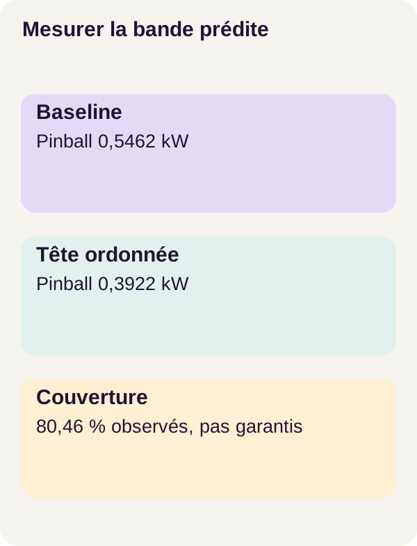
| Ordered head | 0.3922 | 1.2313 | 80.46% | 3.9824 | 0% |
Here, both networks reduce pinball loss and median error compared with the seasonal reference. They also produce narrower bands while maintaining overall coverage close to 80%.
The ordered head is slightly better than the independent head on pinball loss and MAE. To put ‘slightly’ into perspective, the pinball difference is 0,3939 − 0,3922 = 0,0017 kW, and the MAE difference is 1,2350 − 1,2313 = 0,0037 kW. These are subtractions of the published values, not new measurements.
The ordered head’s width is 5,4649 − 3,9824 = 1,4825 kW smaller than the seasonal baseline’s. However, concluding that ‘higher coverage means a better model’ would be misleading: nominal coverage remains 80%, and all three methods are close to that on this sample.
All three methods have zero observed crossings. The table therefore does not demonstrate the correction of crossings actually present in the independent variant. The difference is structural: ordering is enforced in the ordered head, whereas the independent head’s zero describes only this evaluation.
Deterministic resumption recovers the same parameters with zero maximum error, along with the scaler and shared initialization. This result concerns controlled reproduction of the computation. The PyTorch reproducibility documentation explains why a local match should not become a guarantee across all versions and platforms.
What we have learned
We can now replace a single forecast with three learned thresholds and interpret the accompanying band. Pinball loss teaches the quantiles different behaviors; softplus enforces their order; metrics then check how these outputs perform on held-out data.
Time-related discipline applies at several levels. History must be available at the forecast origin, targets must remain within their data split, the scaler must not learn from the future, and the causal block must not use a later position to calculate an earlier output.
In this experiment, the ordered model is slightly better on pinball loss and MAE, with a narrower band than the seasonal reference. This finding does not automatically make it the best production choice. No post-hoc calibration, seasonal drift assessment or analysis of the business cost of underprediction has been validated.
The useful conclusion is therefore not ‘this network can forecast real load’, but: we have a controlled walkthrough for training, resuming and comparing quantile forecasts without confusing ordering, accuracy and calibration.
Exercise: form a hypothesis before running a command
Let us return to padding. We will change an input value at time 10, then examine the outputs assigned to times 0 through 9.
Before running anything, write down your hypothesis: is a causal block allowed to change a past output after this modification? And can a symmetric convolution let the value at time 10 influence the computation at time 9?
The provided check compares both variants. Run it without replacing the network in the reference walkthrough:
docker compose run --rm gpu python -m quantile_forecast.cli exercise --config configs/exercise.yaml
The observed output gives 0,0 for the causal block’s past-output error and 1,0 for the symmetric variant. The former remains unchanged at the examined positions; the latter allows influence from a later position through. The test therefore does detect leakage from the future into the past within the block.
This 1.0 is not a 100% forecasting error rate: it is the difference value reported by this perturbation check.
An important nuance: which future are we talking about? Time 10 is in the future relative to outputs 0 to 9 of the block. If it already belongs to the 168 hours known at the forecast origin, reading it is not by itself proof that the 24 future targets were used. The test checks the block’s internal causality; the window check separately verifies the boundary between history and the horizon to forecast.
To explain the result, return to a centred filter that reads 8, 9, and 10 to calculate output 9. Compare it with a three-position causal filter that would read only 7, 8, and 9. Reading these dependencies is more useful than simply saying “the test passes.”
Adapting and putting into production
Replacing the simulator without losing the temporal contract
With real data, begin by defining what each row represents: the site, timestamp, unit, and expected frequency. A missing value is not automatically a zero load. A measurement received late was not necessarily available at the time your forecast should have been made.
You therefore need authorised, versioned data, an explicit strategy for late and missing values, and a verifiable temporal split. Evaluate what the system knew on the forecast date, not what a database corrected afterwards makes visible today.
The tutorial does not validate these choices on operational data. An adaptation is a new experiment: keep the r1 outputs, work in a copy, and document every change to data, frequency, horizon, or model.
Connecting bands to a decision
A dashboard can display a median and a band without triggering an action. As soon as an action depends on a bound, you must specify the cost of underforecasting, overforecasting, and an unnecessary alert.
The q90 level is not a universal policy of caution. An application may need another level, human validation, or a rejection rule when the band becomes too wide. These are business choices to define and test, not guarantees provided by softplus.
You will also need to check calibration by segment and monitor drift, that is, changes in data and errors over time. Good coverage obtained in the controlled world of the simulator is not enough when habits, equipment, or conditions change.
Building the service around the model
The web side remains work in its own right: authenticated access, permissions by site, input validation, suitable logging, load and error handling, observability, backup, and restoration. Alert thresholds and the action associated with each band must be explicit.
The code provides a teaching path for forecasting. It provides neither a certified forecast nor a business API ready to deploy.
Troubleshooting and cleanup
If CUDA fails, start with the environment check and the NVIDIA Container Toolkit guide. Check access to the selected card from the container before changing the model.
If the causality check fails, inspect the padding and the positions read. Do not change the score to make the failure less visible. If coverage is surprising even though the quantiles are ordered, it is not necessarily an ordering problem: check the targets, units, scaler, and population evaluated.
After the exercise, generate the figures, check the checkpoints, preview cleanup, then stop the services:
docker compose run --rm gpu python lesson/figures/plot.py
docker compose run --rm gpu python scripts/check_checkpoints.py
docker compose run --rm gpu python scripts/clean.py --scope generated --dry-run
docker compose down --remove-orphans
plot.py produces the track’s figures and check_checkpoints.py checks its checkpoints. The command with --dry-run is a preview: it keeps generated files. Read what it reports before considering a separate deletion.
The final command stops the project’s Compose resources. It does not replace the preview with an actual cleanup of your results. Keep useful outputs to compare your experiments.
Primary sources and documentation
The tutorial’s starting references describe the mechanism and its environment:
- Bai, Kolter, Koltun — Temporal Convolutional Networks
- Scikit-learn — pinball loss
- Docker Compose — GPU support
- NVIDIA Container Toolkit — installation guide
For more detailed explanations, the PyTorch reference for softplus details the increments, and the broadcasting rules explain the move from one target per hour to three comparisons.
The scikit-learn example on prediction intervals uses another model: it complements the explanation of quantiles without serving as evidence for our TCN’s results. The page on data leakage explores the role of preprocessing, and the PyTorch documentation on reproducibility specifies the limits of reproductions across environments.
This article’s experimental values remain those of the r1 track. Numerical examples marked as teaching examples are used to repeat calculations; they are not new GPU outputs.
Download the archive and follow the complete track: open the tutorial.