





Imagine a customer-support inbox. Your application needs to route each message to the right category: an invoice to locate, an incident to resolve, an access problem, or a request for information. You already know how to receive a message, validate JSON, and save the result. Here we will explore the part that turns free text into a usable category.
Take this teaching example, invented to illustrate the need: "Since this morning, the payment page has returned a 500 error." We would like a response like this:
{
  "label": "INCIDENT",
  "explication": "Le message signale une erreur technique sur la page de paiement."
}
This message and this JSON are neither a corpus row nor a measured output. They simply show the expected contract: one of four classes, accompanied by a short explanation.
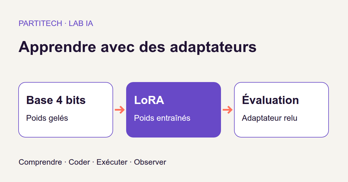
We already have a local language model. Rather than reteaching it how to write, we will adapt a small part of its parameters to this task. The method is called QLoRA. We will understand how it works, follow the code, reproduce the training run, and then examine what the scores really demonstrate.
The goal is not to promise a universally better model. It is to answer two separate questions: did training actually change anything, and does that change improve what our application needs?
Download the complete tutorial project. The base weights are not included: acquisition downloads them and then checks their size and SHA-256 digest. The commands in this article match the r3 run; the explanatory examples do not alter that protocol.
Vocabulary to understand before running the code
A pretrained base, not a model built from scratch
A language model uses parameters, also called weights: numerical values that influence the text it produces. The name 7B indicates a size of roughly seven billion parameters. It does not mean seven billion searchable documents or seven gigabytes of memory.
The base here is the model before our adaptation. It already knows how to generate text; we want it to produce the responses expected for our task. Adapting an existing model from examples is fine-tuning. We are not performing its original pretraining.
Changing only the instruction sent to the model, the prompt, does not change its weights. Full fine-tuning would update all weights involved in training. In this tutorial, we take another route: keep the base and learn small additional parameters. That is the principle of parameter-efficient adaptation methods documented by PEFT.
This choice lets us study adaptation with a smaller memory footprint. It does not prove that training is needed for every classification task: comparison with the unadapted base remains essential.
Learning from messages and expected answers
Supervised learning consists of providing an input and the answer we want to obtain. Here, the input is a message; the target is JSON containing label and explication. The four allowed classes are FACTURE, INCIDENT, ACCES, and INFORMATION.
The model does not handle our character strings directly. A tokenizer splits text into units, tokens, then turns them into numerical identifiers. A token is not necessarily a whole word.
During training, the model assigns probabilities to the next tokens. The loss, called loss in the code, penalizes predictions that give too little probability to the expected tokens. It is a numerical learning signal, not yet a business-quality score.
Backpropagation, triggered by backward(), calculates how that loss changes with the trainable parameters. Those changes are the gradients. The AdamW optimizer uses them to adjust parameters. An optimization step is one update; it is not necessarily an update after every message.
Remember the chain: the model predicts, the loss measures the gap, gradients show how to act, and the optimizer makes the change.
QLoRA: storing the base more lightly and learning an adapter
LoRA, short for Low-Rank Adaptation, adds small trainable matrices to targeted model layers instead of changing their original weights. A matrix here is a table of numbers; a linear layer uses such tables to transform numerical representations of text. The method is described in the LoRA research paper.
You can think of the adapter as a learned correction added to the base's behavior. It is neither a new prompt nor a list of if/else rules: it consists of real numerical parameters.
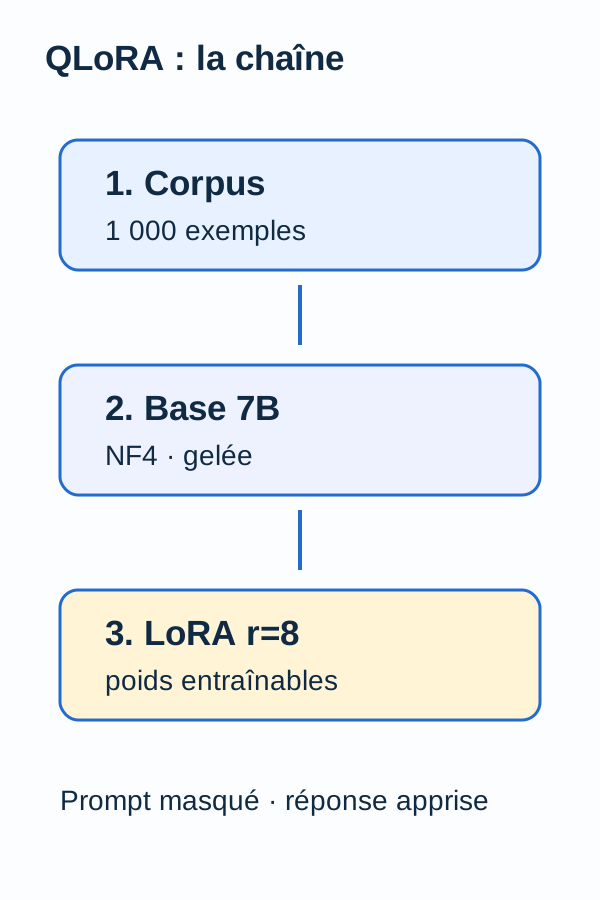
QLoRA combines these adapters with a quantized base. Quantization uses fewer bits to represent the selected weights, reducing their memory footprint. In our experiment, the base is loaded in 4 bits, in NF4 format, with double quantization. NF4 is a representation designed for weights whose distribution is close to a normal distribution. Double quantization also reduces the space used by the coefficients of that representation; it does not mean two successive training runs. These mechanisms are presented in the QLoRA paper.
Keep one essential distinction in mind: storing weights in 4 bits does not mean performing every calculation in 4 bits. Here, computation in quantized layers is configured as bfloat16, a 16-bit numerical format. The Transformers documentation on bitsandbytes clearly distinguishes quantized storage from computation type.
The base weights remain frozen: they still take part in calculations, but the optimizer does not update them. Only the LoRA adapters are trained. Their settings in this project are:
| Setting | Tutorial value | What it controls |
|---|---|---|
Rank, r |
8 |
The internal dimension of the small correction matrices. It is not the number of classes. |
lora_alpha |
16 |
The scale of the adapter contribution. |
lora_dropout |
0.0 |
No dropout in the LoRA branch: no random deactivation for this reason. |
target_modules |
all-linear |
Eligible linear modules selected by PEFT. This does not make every base weight trainable. |
In the standard LoRA formulation, the scale uses alpha / r, so 16 / 8 = 2 here. That does not mean "twice as accurate." The details and selection rules for all-linear are specified in the LoraConfig reference. To reproduce the experiment, keep the ZIP values rather than those from another documentation example.
The model reads the instruction, but we score its answer
Imagine an exercise with a question and an answer to write. The student must read the question; the grade concerns the answer, not their ability to copy the instructions.
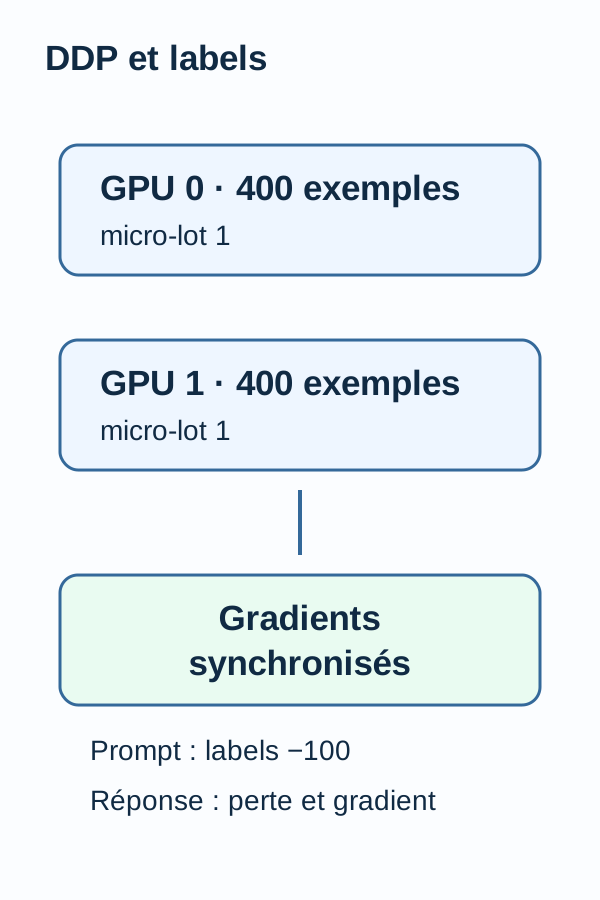
The same principle applies here. The encode() function keeps the prompt in the input, but marks its positions with -100 in the training targets, labels. Those positions are ignored in the loss. Ignored for scoring does not mean hidden from the model. We will see this mechanism in the code.
Two GPUs: sharing examples, not merging memory
DDP, short for DistributedDataParallel, runs several replicas of the model while synchronizing their gradients. In this project, two processes each use an RTX 3090. Each card carries its own replica: we are not creating an imaginary 48 GiB card.
Each GPU processes 400 of the 800 training examples. The micro-batch is 1: one example at a time on each card. Gradient accumulation is 4: each process accumulates the work of four examples before the shared update.
The number of examples contributing to one step is therefore 1 × 2 × 4 = 8. For 800 examples, that gives 800 / 8 = 100 optimization steps. These are not 100 complete passes through the corpus.
After every update, the protocol checks that the maximum difference between the monitored replicas is zero. The PyTorch DDP documentation describes this synchronization and notes that data partitioning remains the program's responsibility.
Data and pipeline
The corpus contains 1,000 synthetic examples, distributed across the four classes. "Synthetic" means we are studying a set built for the experiment, not a sample of real requests validated by a customer-support team.
The data is divided into three sets, often called splits:
| Set | Number of examples | Role in the experiment |
|---|---|---|
Training, train |
800 | Provides the examples used for updates. |
| Development | 100 | Observes loss on examples separate from training. |
| Test | 100 | Compares outputs from the base and the reloaded adapter. |
The separation is not only between rows: message families do not overlap across sets. To understand why this matters, imagine two identical requests whose only difference is an invoice number. Putting one in training and the other in testing could create an exaggerated impression of novelty. This example illustrates the risk; it does not describe a specific corpus family.
We speak of data leakage when information that should remain reserved for evaluation artificially helps learning or model selection. Here, validate_data() checks identifiers, the 800/100/100 sizes, labels, text, and the absence of family overlap before loading the model. It is the equivalent of validating data before an expensive process.
The pipeline, meaning the sequence of processing steps, follows this order: validate the data, evaluate the base alone, prepare the NF4 base for training, then add LoRA. Next we train the adapters, check gradients and modified weights, save the adapter, and reload it onto a new base before evaluating again.
Why insist on reloading? A result obtained with an object still in memory is not enough to show that the saved file works. The model evaluated after adaptation must use the adapter read back from disk.
Among other things, train.py rejects invalid data, family leakage, a context longer than 1,024 tokens, or a missing adapter. These negative tests check that bad inputs are rejected. As with an API, success in the nominal case is not enough.
Core functions to read before running
The following four excerpts show the essential mechanisms. They do not form a standalone script: imports, distributed initialization, the tokenizer, data, and the other functions are in the complete project. Use the archive commands to run the workflow.
In these excerpts, RANK identifies the process and its card in this two-GPU setup; WORLD is 2, the number of participating processes. tok is the tokenizer and DATA contains the loaded corpus.
Loading the local base in 4 bits
load_base() reads weights from /models/qlora, a path inside the container. The configuration requests NF4, double quantization, and bfloat16 computation.
quant = BitsAndBytesConfig(
    load_in_4bit=True,
    bnb_4bit_quant_type='nf4',
    bnb_4bit_use_double_quant=True,
    bnb_4bit_compute_dtype=torch.bfloat16,
)


def load_base():
    m = AutoModelForCausalLM.from_pretrained(
        '/models/qlora',
        local_files_only=True,
        quantization_config=quant,
        device_map={'': RANK},
        torch_dtype=torch.bfloat16,
        attn_implementation='sdpa',
    )
    assert m.is_loaded_in_4bit
    m.config.use_cache = False
    return m
local_files_only=True prevents this loading step from fetching missing files online. Acquisition is a separate step. device_map={'': RANK} places this replica on the card associated with the process: it is not automatic model sharing between the two cards.
The m.is_loaded_in_4bit assertion checks that 4-bit loading took place; NF4 is requested by the configuration immediately above. On its own, it is not an audit of every internal parameter. use_cache=False disables the generation cache in this training workflow; attn_implementation='sdpa' retains the attention mechanism selected in the tested environment.
What we have just done: load the base, not train it yet. Preparing it for quantized training and adding adapters belong to the next stages of the complete program.
Turning an example into an input and a target
The encode() function prepares what the model will read and the positions on which to calculate loss.
def encode(row):
    answer = json.dumps(
        {'label': row['label'], 'explication': row['explanation']},
        ensure_ascii=False,
    )
    a = tok(prompt(row), add_special_tokens=False)['input_ids']
    b = tok(answer + tok.eos_token, add_special_tokens=False)['input_ids']
    ids = a + b

    if not 0 < len(ids) <= 1024:
        raise ValueError('context >1024')

    return {
        'input_ids': torch.tensor([ids], device=RANK),
        'attention_mask': torch.ones(
            (1, len(ids)),
            device=RANK,
            dtype=torch.long,
        ),
        'labels': torch.tensor([[-100] * len(a) + b], device=RANK),
    }
Let us start with the names. In the source data, the explanation is called explanation. The JSON we want to learn uses the French key explication. The first line of the function makes that correspondence without changing the expected class.
a contains the identifiers for the instruction and message. b contains those for the expected JSON, followed by eos_token, the end-of-sequence marker. ids = a + b forms the complete sequence.
To visualize masking, take made-up identifiers unrelated to the real tokenizer:
Prompt :       [11,   12,   13]
Réponse :      [21,   22]
input_ids :    [11,   12,   13, 21, 22]
labels :       [-100, -100, -100, 21, 22]
Prompt identifiers remain in input_ids, but are replaced with -100 in labels. The ignore_index=-100 convention of PyTorch cross-entropy loss makes it possible to ignore those targets. It is neither a minus-one-hundred penalty nor a token to generate.
Why does the answer also appear in the input during training? In a causal language model, each position learns to predict the next token from the preceding ones, with no access to later tokens. The model handles the shift between predictions and targets. In use, the expected answer is no longer provided: the model generates it. The Hugging Face course on causal models explains this mechanism.
Here, attention_mask is filled with 1 for positions that are present. Do not confuse it with loss masking in labels, or infer that the model can read future tokens.
Finally, the 1,024-token limit applies to the whole prompt + answer + end marker. The program rejects an out-of-range sequence instead of silently cutting the answer. This limit belongs to the tested protocol; it does not necessarily describe the model's maximum capacity in other uses.
Adding LoRA and performing updates
get_peft_model() adds the adapters. The trainable list retains only parameters whose requires_grad is true, then an assertion requires their names to contain lora_. In other words, the program checks what it allows to learn before optimization starts.
A tensor is a numerical array that can have several dimensions. before copies trainable tensors before the first update; initial_hash calculates a digest of their bytes. Together, they make it possible to compare the initial and trained states.
model = get_peft_model(
    base,
    LoraConfig(
        r=8,
        lora_alpha=16,
        lora_dropout=0.0,
        target_modules='all-linear',
        bias='none',
        task_type='CAUSAL_LM',
    ),
)
model.config.use_cache = False
trainable = [p for p in model.parameters() if p.requires_grad]
assert trainable and all(
    ('lora_' in n for n, p in model.named_parameters() if p.requires_grad)
)
before = [p.detach().cpu().clone() for p in trainable]
initial_hash = hashlib.sha256(
    b''.join((p.numpy().tobytes() for p in before))
).hexdigest()

# Répliques DDP :400 exemples par GPU, accumulation4, batch global8.
wrapped = DDP(
    model,
    device_ids=[RANK],
    output_device=RANK,
    find_unused_parameters=False,
    broadcast_buffers=False,
)
optimizer = torch.optim.AdamW(trainable, lr=0.0002, weight_decay=0.01)
train = [q for q in DATA['queries'] if q['split'] == 'train']
random.Random(42).shuffle(train)
own = train[RANK::WORLD]
assert len(own) == 400
partitions = [None] * WORLD
dist.all_gather_object(partitions, [q['id'] for q in own])
emit('training-partition', rank_ids=partitions)
accum = 4
losses = []
start = time.monotonic()
optimizer.zero_grad(set_to_none=True)
wrapped.train()
maxnorm = 0

for i, row in enumerate(own):
    sync = (i + 1) % accum == 0
    with contextlib.nullcontext() if sync else wrapped.no_sync():
        loss = wrapped(**encode(row)).loss
        assert torch.isfinite(loss)
        (loss / accum).backward()

    losses.append(float(loss.detach()))
    if sync:
        norm = torch.nn.utils.clip_grad_norm_(trainable, 1.0)
        assert torch.isfinite(norm)
        maxnorm = max(maxnorm, float(norm))
        optimizer.step()
        optimizer.zero_grad(set_to_none=True)
        both = torch.tensor(sum(losses[-4:]) / 4, device=RANK)
        dist.all_reduce(both)
        emit(
            'train-step',
            step=(i + 1) // 4,
            loss=float(both) / WORLD,
            rank0_example_ids=[r['id'] for r in own[i - 3:i + 1]],
            gradient_norm=float(norm),
        )
The excerpt is longer, but it follows three familiar operations: distribute work, perform it, then log what happened.
Distribute examples. random.Random(42).shuffle(train) shuffles data with a fixed seed. train[RANK::WORLD] then takes every other row: one process handles even positions, the other odd positions in that shuffled list. Each must receive exactly 400 examples. all_gather_object() collects their identifiers for the training-partition event.
Accumulate, then update. For every example, wrapped(**encode(row)).loss calculates loss. The isfinite assertion rejects an infinite or undefined value. (loss / accum).backward() accumulates the gradient contribution after dividing it by 4. The first three examples use no_sync(); the fourth triggers synchronization before the update. This is the accumulation mechanism described in the DDP.no_sync() documentation.
clip_grad_norm_(trainable, 1.0) limits the global gradient norm, a measure of their magnitude, to prevent an update driven by gradients that are too large. The returned and logged value is the norm before that limit: a value above 1 in the log does not automatically mean the check failed. See the PyTorch reference for clip_grad_norm_.
optimizer.step() then applies the update. The AdamW optimizer uses lr=0.0002, the learning rate that sets the scale of adjustments, and weight_decay=0.01, a weight regularization term. zero_grad(set_to_none=True) resets gradients for the next group. The project uses torch.optim.AdamW exactly as shown, not another optimizer substituted for the validated workflow.
Logging. The final lines calculate an average loss and record it with the step number and gradient norm. The explicit call to dist.all_reduce(both) aggregates the loss for the log here: DDP synchronizes gradients during backpropagation.
The checks after this loop in the complete program require modified weights, nonzero gradients, and identical replicas. They are not all reproduced in this excerpt. After saving, adapter_hash() reads the LoRA parameters back: an identical digest before and after reload checks that the adapter being evaluated is the one that was saved. Like an artifact checksum, SHA-256 checks the identity of compared bytes, not the quality of responses.
Counting correct answers without hiding format errors
The classification() function in metrics.py reads generated outputs and compares them with expected classes. Here is its decoding and counting section; final calculation and returned metrics are in the complete ZIP function.
def classification(rows, expected):
    matrix = [[0] * 5 for _ in range(4)]
    correct = 0

    for row in rows:
        truth = LABELS.index(expected[row['sample_id']]['label'])
        try:
            obj = json.loads(row['raw'])
            label = obj['label']
            pred = (
                LABELS.index(label)
                if isinstance(obj.get('explication'), str)
                and obj['explication'].strip()
                else 4
            )
        except (ValueError, KeyError, TypeError):
            pred = 4

        matrix[truth][pred] += 1
        correct += pred == truth
matrix has four rows, one for each actual class, and five columns: the four possible classes plus an error column. An invalid answer therefore remains in the report; it is not removed to make the score look better.
The code first decodes row['raw'] with json.loads(). It then looks for the label value in LABELS. To accept that prediction, explication must be a nonempty string after leading and trailing spaces are removed. Errors handled by except are counted in the fifth column.
Notice the detail: strip() is applied to the explanation, but not to the label in this strict evaluation. A label with a trailing space therefore does not match the allowed value without that space.
That does not mean the program compares every byte of JSON. Indentation spaces are accepted by the parser; a space inside the label value, however, changes the string being compared. We will return to this distinction in the exercise.
Keep another limitation in mind: this check verifies that the explanation exists and is not empty. It judges neither its relevance, truthfulness, nor brevity. The presence of text is not validation of its content.
Reproducing the workflow in order
To follow the practical section, you need to be able to read Python, use a terminal, and recognize a JSON object. Scripts run from the root of a fresh archive extraction; do not rebuild the project by assembling only article excerpts.
The validated profile uses Linux x86_64, Docker/Compose, an NVIDIA driver and NVIDIA Container Toolkit, with two RTX 3090s. The stated provisions are 48 GiB RAM, 40 GiB disk, and 20 GiB free VRAM on each card. RAM belongs to the machine; VRAM is each GPU's memory. These values are provisions, not measured minimums.
No CPU workflow has been validated. The program requires two GPUs for this reproduction; reducing their number is not a simple variation of the same run.
1. Check the host, then prepare the image
The preflight is a prerequisite check. It must confirm Docker, Compose, both cards, and CUDA access from a container. CUDA is the NVIDIA compute environment used by this stack; seeing the cards on Linux does not show that Docker can use them. The NVIDIA Container Toolkit guide describes how to configure that access.
./scripts/preflight.sh
sh scripts/setup.sh
docker compose build
setup.sh prepares the local permissions used by Compose. docker compose build then builds the project image.
What to observe: checks pass and the build finishes without an error. If the GPU is visible only from the host, fix Docker access before acquisition and training.
2. Acquire the base and check safeguards
The fetch service downloads a pinned model revision, checks its size and SHA-256, then places the final file. Here, a pinned revision plays the role of a precise dependency version: it lets you know exactly which files were used for the experiment.
docker compose --profile acquisition run --rm --no-deps fetch
docker compose run --rm --no-deps app -m unittest discover -s tests -v
The second command runs the test suite. It covers, in particular, negative cases relating to data and context.
What to observe: 15 public tests pass. A hash failure is not a warning to bypass. A different model retrieved from an unidentified cache would no longer reproduce the described experiment.
3. Prepare, then train the adapter
prepare validates the corpus and produces prepared data. train evaluates the base, performs the 100 DDP steps, and reloads the adapter. This is the stage that uses both GPUs.
docker compose run --rm --no-deps app -m src.cli prepare
docker compose run --rm --no-deps app -m src.cli train
What to observe: JSON events training-complete, adapter-roundtrip, and complete, with 800 examples, 100 steps, and replica_max_difference equal to 0.
The round-trip is saving and then reloading. If this event is absent, do not conclude that the reloaded adapter was evaluated correctly. A falling loss in the log does not replace this verification.
4. Produce metrics
We can now build the classification report and confusion matrices.
docker compose run --rm --no-deps app -m src.cli evaluate
What to observe: one classification JSON for the base and another for the reloaded adapter. Before running exercise, take time to understand the scores below: the exercise will ask you to predict the effect of a change in how results are read.
How to read the metrics before the results
Accuracy and macro-F1: two complementary views
Accuracy is the proportion of examples correctly classified under the program's rules. A score of 0.90 on 100 cases means 90 answers meet those rules. Here, a format error or empty explanation is enough to fail a case.
F1 combines two ideas. For a given class, precision asks: "Among answers that announce this class, how many are correct?" Recall asks: "Among messages that actually belong to this class, how many were found?" F1 is their harmonic mean, calculated as 2 × precision × recall / (precision + recall) when the denominator is nonzero.
Macro-F1 calculates an F1 for each of the four classes, then averages them. Each class therefore has the same weight in that average, whatever its population. The scikit-learn metric documentation expands on these definitions; this tutorial's score is still calculated by its own metrics.py module.
The confusion matrix then helps explain errors. It crosses expected class with predicted class, while retaining an extra column for rejected outputs. Confusing FACTURE with INCIDENT does not tell the same story as an INCIDENT answer rejected because of a trailing space.
Low loss does not replace these checks
Development loss measures how closely the model's probabilities match expected tokens in the development set. It is neither a percentage of business errors nor an independent measure of explanation quality.
Moreover, a good score is not enough to prove that the training chain worked as intended. The project separately checks 392 modified LoRA tensors, 20,185,088 trainable parameters, 100 optimization steps, nonzero gradients, and equality of adapters on both replicas.
The first two numbers do not count the same thing: tensors are the arrays; parameters are the numerical values they contain. The checks establish that adapters were modified and synchronized; scores then show how their outputs behave on the corpus.
Observed results, and what they allow us to conclude
The following values are those reported for the r3 workflow. Evaluation covers the 100 test cases, not the 800 examples used for updates.
| Test measurement | Unadapted base | Base with reloaded adapter |
|---|---|---|
| Strict accuracy | 0.90 | 1.00 |
| Macro-F1 | 0.9167 | 1.00 |
INCIDENT cases in the format-error column |
10 | 0 |
At first glance, the move from 0.90 to 1.00 seems to tell a simple story: "We taught the model to classify better." But the matrix calls for a more precise reading. The base's 10 failures are in the format-error column, not in another business class.
The conclusion directly supported is therefore that the reloaded adapter better meets this experiment's strict contract. We cannot turn this result into evidence of a better understanding of incidents, especially because the exercise shows the effect of cleaning the base labels.
Training lasted 139.5 s in the first reproduction and 141.6 s in the second. These times concern the reported training, not a promise of total time including installation and download. Observed development loss was 1.4785609673708677e-05, or about 0.0000148: that decimal notation is a rounded conversion of the same value, not a new measurement.
Recorded VRAM maxima were about 14,145 MiB and 13,722 MiB, depending on the GPU. Memory was sampled about once a second: a peak between samples may escape measurement. These values therefore do not replace the stated provision of 20 GiB free per card for reproduction.
These results describe this corpus, these settings, and this machine. They demonstrate neither generalization to real messages, superiority over another model, nor production quality. Public Docker caches and the computer's general activity are also part of the observed resource context.
What we learned
We followed a complete chain: data separated by family, a quantized and frozen base, trainable LoRA adapters, synchronized gradients, saving, then reloading onto a new base. Training is not just a loss curve: you must also know which parameters changed and which artifact was evaluated.
We also distinguished learning from measuring. Changing weights changes model behavior. Changing how its outputs are read can change a score without touching the model.
The adapter's 1.00 score remains a result on 100 synthetic test cases. Moving the base from 0.90 to 1.00 after removing spaces is another operation: its responses are the same, but their comparison becomes more forgiving. Confusing the two would mean claiming a semantic improvement the experiment does not establish.
Active exercise: predict, change, run, observe, explain
You are now on the developer's side, receiving JSON. Before running the command, consider these two objects, built for explanation rather than copied from a screenshot:
{
  "label": "INCIDENT",
  "explication": "Un problème technique est signalé."
}
{
  "label": "INCIDENT ",
  "explication": "Un problème technique est signalé."
}
Both objects are valid JSON. Yet in the second one, the label value has a trailing space. Predict what LABELS.index(label) will do, then what would change if it compared label.strip().
Python's strip() method removes whitespace characters from the beginning and end of a string; it does not retrain the model or turn a wrong business class into the right one.
Now run the supplied exercise. The change being studied concerns how labels are read, not the model's weights:
docker compose run --rm --no-deps app -m src.cli exercise
Results to observe: strict baseline 0.90; baseline with cleaned label 1.00. Here, baseline means the comparison reference, namely the unadapted base.
A tempting hypothesis would be: "The score rises, so the model understands messages better." The result does not confirm it. No weights changed; the exercise reveals sensitivity to formatting.
State your conclusion this way instead: "The base labels meet the comparison after normalization. This forgiving score must be reported separately from the strict score." Normalization can be useful in an application, but it must not silently erase the evaluated contract.
To check that you understand, explain why the same operation would not correct a FACTURE label assigned to a message that is actually INCIDENT. You will then have distinguished a format correction from a classification correction.
Troubleshooting and cleanup
Only one card is visible. Check GPU_DEVICE and GPU_DEVICE_2, then start again with preflight. If WORLD_SIZE or the number of GPUs is not 2, training deliberately stops. The distribution of 800 examples and the global batch described above rely on this contract.
A sequence exceeds 1,024 tokens. Check the total length of the instruction, message, answer, and end marker. In a separate experiment using your own examples, shorten the example rather than silently truncating its answer. If the reference corpus triggers this error, first check the files and reproduction configuration before changing them.
The adapter does not reload. Check the outputs/artifacts/adapter directory and start again from a fresh extraction, not an assembly of partial files. Without a validated reload, adapted evaluation cannot be interpreted as an evaluation of the saved artifact.
At the end of the workflow, from the project root, stop Compose resources:
docker compose down
This command removes neither models nor outputs. Keep the results needed for your comparison. To remove your working files, delete only the extraction folder you created after checking its contents, not resources shared with other projects.
Going further
The interesting next step is not to seek a more spectacular score immediately. It is to build a test where an error can no longer be resolved by simply removing a space.
In a separate experiment, retain the principles of this protocol and replace the synthetic corpus with an annotated set representative of your messages. Keep separation by client, family, or period to avoid finding variants too close to training examples in the test. Always compare the unadapted base and adapter on the same prompts and cases.
Also plan for abstention: an answer meaning that the system cannot classify a message acceptably and must pass it to a person. This possibility is not one of the four current contract classes; adding it requires changing data, expected format, validation, and metrics, then measuring again.
Have people who know the business review the matrix errors and explanations. Distinguish format errors, wrong categories, and incorrect justifications. These extensions are not results already obtained by r3: they define the work needed to measure usefulness beyond our controlled example.
Limits before real-world use
The set is synthetic and small, the test has 100 cases, and no independent human review is claimed. A very low loss and a perfect score on this test do not validate ambiguous messages, unexpected wording, or the quality of explanations in your application.
DDP synchronizes learning across two GPUs; by itself, it does not provide a deployment strategy. Before any business decision, you need representative data, rejection criteria, a review of errors by class, and independent evaluation, with time- or client-based separation suited to the need.
Also retain the version of the corpus, base model, tokenizer, dependencies, calculation rules, and adapter. Comparing two scores is meaningful only when you know what changed between the two experiments.
The official PEFT documentation on quantization goes further into combining a quantized base with trainable adapters. This article's references explain the mechanisms; they do not replace the pinned versions and parameters in the ZIP needed to reproduce this tutorial.