





You are developing a back office where a team uploads and classifies documents. A service report arrives: should it go under Maintenance, Quality, or both? A single-choice dropdown is no longer enough. You need multiple labels organized in a tree.
A DMS, or document management system, can face exactly this problem. The same item may belong to maintenance/interventions and qualite/controles. The filing plan must also be respected: proposing qualite/controles without including its parent qualite produces an inconsistent suggestion.
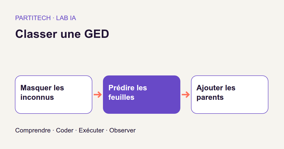
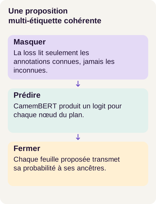
We will train CamemBERT on the fictional Vesta corpus to propose these classifications. The workflow is: text → numerical representations → category scores → proposals compatible with the hierarchy. The prototype moves no files and grants no access rights. It prepares a suggestion for confirmation.
Download the r001 tutorial ZIP
We will follow case D-031 to inspect the mechanism. This example comes from training; its annotations are accessible for explanation. The 360 test documents will be evaluated separately.
The main trap resembles a common form error: an unanswered box does not necessarily mean “no.” In training, confusing an unknown annotation with a negative answer would teach the model something nobody has established. The final exercise will show the consequences of this confusion.
Vocabulary and metrics before the code
A taxonomy: categories and their relationships
A taxonomy here is the classification plan. Each category is a node. A category can have children: achats is the parent of achats/factures. A category with no children is a leaf. A node's ancestors are the categories encountered when moving toward the top of the tree.
The project has 12 leaves, but the model also produces scores for parents. There is therefore one output per taxonomy node, not just twelve outputs.
Classification is multi-label: several categories can be true for one document. Think of multiple checkboxes rather than radio buttons imposing a single choice. The leaves maintenance/interventions and qualite/controles are not necessarily competitors.
The hierarchy adds a constraint: a proposal for qualite/controles must include qualite. Conversely, proposing qualite does not require proposing all its leaves. A parent is not a shortcut for selecting every child.
From text to numbers: CamemBERT's role
CamemBERT is a model pretrained on French text. We use it as an encoder: it transforms a text sequence into numerical representations. It does not write conversational responses in this project. The Hugging Face CamemBERT documentation explains how it works and its classification uses.
The tokenizer first divides text into units called tokens. A token may correspond to a piece of a word; it is not necessarily a whole word. The tokenizer converts these units into identifiers and adds special tokens to structure the sequence.
The encoder then produces a vector for each position: a list of numbers representing that position in the context of surrounding text. These numbers are features computed by the model, not directly readable categories such as “invoice” or “inspection.”
Pretrained does not mean it already knows our classification plan. Adaptation using Vesta annotations teaches it the intended document task: this is fine-tuning, or adapting a pretrained model to a task. Weights are numerical parameters adjusted during learning; they are not a list of documents to consult.
To process several documents together, we form a batch. Because sequences differ in length, shorter ones receive padding. The attention mask indicates which positions to consider and which are padding. Special sequence tokens are not automatically padding: the mask makes the distinction. The Transformers glossary explains this concept.
Average without letting padding decide
Our classifier expects one vector per document, not a variable number of vectors. The project therefore uses masked pooling: it averages representations of valid positions.
Consider a two-dimensional illustration unrelated to any measured CamemBERT output. Three valid positions have vectors [2 ; 4], [4 ; 2], and [6 ; 6]. Their sum is [12 ; 12], so their mean is [4 ; 4].
Add two padding positions, represented by [0 ; 0] for simplicity. Averaging all five positions would give [2.4 ; 2.4]. The content has not changed, but its representation would be artificially reduced. Exclude padding from the sum and divide by the number of valid positions. In practice, do not assume that representations computed at padding positions are zero either.
The arrays handled by PyTorch are called tensors. With B documents, T positions per sequence, and H numbers per vector, representations have shape B × T × H. Pooling produces B × H. The classification head, the part that turns this vector into category scores, finally produces B × K, where K is the total number of nodes.
A logit, a probability, and a decision are three different things
Each head output is a logit: a raw number that can be negative or positive. The sigmoid transforms it using p = 1 / (1 + exp(-z)), where z is the logit and exp the exponential function. For example, logits -2, 0, and 2 yield approximately 0.1192, 0.5, and 0.8808 respectively. The formula is documented by PyTorch for Sigmoid.
This transformation is applied to each category. Two leaves can receive high scores: their probabilities do not have to sum to 1, because multiple memberships can be true simultaneously.
A decision rule is then needed to turn scores into proposals. A threshold of 0.5 will be used in our numerical examples solely to simplify calculations; it does not replace the r001 configuration. Likewise, a score of 0.8 alone does not demonstrate that eight out of ten comparable suggestions will be correct.
After sigmoid transformation, ancestor closure propagates child scores upward to parents by taking the maximum. It makes scores compatible with the hierarchy. It does not modify the logits used for learning or turn a wrong category into a correct one.
An annotation has two pieces of information: its value and whether it is known
An annotation indicates whether a document belongs to a category. This project distinguishes three situations:
| Situation | Target value | Used for learning? |
|---|---|---|
| Confirmed membership | 1 |
Yes. |
| Confirmed non-membership | 0 |
Yes. |
| Unknown membership | Value ignored | No. |
For a web developer, this distinction resembles a nullable boolean: true, false, and missing information. This is an analogy, not a description of a database schema supplied by the project.
The loss function, called loss in the code, measures the gap between model outputs and known annotations. Training adjusts parameters to reduce it. Here, we use binary cross-entropy, or BCE, only on document–label pairs that were actually observed.
Note that we now have two different masks. The attention mask concerns text positions, with shape B × T. The annotation mask concerns known categories, with shape B × K. Removing an annotation from the loss does not remove words from the document.
Measure labels, then the whole document
A true positive is an expected leaf that is proposed. A false positive is a wrongly proposed leaf. A false negative is an expected leaf that is missed. Precision measures correct proposals among those emitted; recall measures expected memberships that were recovered.
F1 combines precision and recall. With VP true positives, FP false positives, and FN false negatives, it is 2 × VP / (2 × VP + FP + FN). Micro F1 combines counts from all leaves before this calculation. Macro F1 calculates F1 for each of the 12 leaves, then takes their unweighted mean. These conventions are described in the f1_score documentation.
A small illustration explains the difference. Suppose there are only two leaves: the first is recovered 90 times out of 90 without error; the second is missed ten times out of ten and never proposed. Micro F1 is 180 / 190, approximately 0.9474. Yet macro F1 is (1 + 0) / 2 = 0.5. Success on a frequent category can therefore hide complete failure on another.
The exact leaf set asks a stricter question: are all this document's leaves correct, with no additions or omissions? The exact node set requires the same for leaves and parents. It compares sets, not display order; multi-label exactness is also explained by scikit-learn.
Finally, the parent–child violation rate examines the plan's consistency: was a child proposed without its parent? A zero rate is desirable, but an entirely wrong branch can still be perfectly consistent.
Prepare the GPU workflow
Check prerequisites and retain the reference configuration
You need to know how to use Python, a terminal, and Docker. PyTorch will perform tensor calculations; the necessary binary classification concepts have just been introduced.
The reference profile is Linux with an RTX 3090 featuring 24 GiB of graphics memory. Also allow 24 GiB of RAM and 35 GiB of working disk space, plus Docker storage. These are preparation recommendations, not guaranteed minimums or usage figures on every machine.
The main workflow uses three epochs: an epoch is one pass over training examples. The exercise will run two new three-epoch training sessions. The r001 validation described here used a GPU; the following commands reproduce that workflow, not an alternative CPU mode. The lexical reference will, however, run on CPU.
The six required public assets are acquired with size and SHA-256 fingerprint verification. This fingerprint identifies the expected contents of a file. No pretrained weights or private repository are included in the ZIP: downloading assets is part of preparation.
Unzip the archive and place your terminal at its root. All commands in the article run from this directory in the order shown. Retain the ZIP's dependencies and configs/minimum.yaml configuration to reproduce r001.
Check the host and build the services
sh scripts/preflight.sh
sh scripts/setup.sh
docker compose config --quiet
docker compose build acquisition tutorial learning inference
The preflight checks Docker, Compose, memory, disk, and GPU. The config --quiet check succeeds without displaying text when the Compose configuration is valid. A silent command is therefore not necessarily one that did nothing.
A GPU visible through nvidia-smi on the host does not yet prove that a program inside Docker can compute on it. NVIDIA Container Toolkit provides container integration. The preflight points to the required documentation if this integration is missing, without changing the system for you. To select another card, set GPU_DEVICE=1 before the workflow.
Acquire files, then test inside Docker
docker compose run --rm acquisition python scripts/acquire.py --config configs/minimum.yaml
docker compose run --rm tutorial python scripts/check_environment.py
docker compose run --rm tutorial python -m pytest -q
Acquisition checks the six files before installing them atomically: this avoids treating a partially acquired file as the final file. check_environment.py then loads the weights and performs a CUDA calculation inside the container. It thus checks actual execution capability, not merely hardware presence.
Tests cover the annotation mask, hierarchical closure, and negative cases among other things. A negative case checks that invalid input is rejected. Do not begin training by bypassing failed checks: understand their cause first.
Create data and make the mechanism inspectable
Prepare Vesta and a comparison method
docker compose run --rm tutorial python -m ged_classement_hierarchique.cli prepare --config configs/minimum.yaml
docker compose run --rm learning python -m ged_classement_hierarchique.cli baseline --config configs/minimum.yaml
docker compose run --rm tutorial python -m ged_classement_hierarchique.cli inspect-mechanism --config configs/minimum.yaml
prepare creates the fictional corpus and its taxonomy. baseline runs a lexical reference, a method based on the project's intended text clues. This comparison answers a useful question: does the network add anything over a simpler solution? The command's use of the learning service does not change this reference's CPU profile.
inspect-mechanism makes case D-031 inspectable. The logits in this demonstration are illustrative and explicitly marked as such. They help trace the calculation; they must not be presented as predictions from an already trained model. The small calculations added below are also independent illustrations, not new measurements on D-031.
masked_bce: select before calculating
Look at the central safeguard. logits contains raw scores, targets the expected values, and mask indicates known document–label pairs.
def masked_bce(logits, targets, mask):
    if (
        logits.shape != targets.shape
        or logits.shape != mask.shape
        or mask.dtype != torch.bool
    ):
        raise ValueError("Expected matching B x labels tensors and a boolean mask")
    count = int(mask.sum())
    if count == 0:
        return None, 0
    # Index first: unknown targets may even be NaN and never enter BCE.
    selected = targets[mask]
    if (
        not torch.isfinite(selected).all()
        or not ((selected == 0) | (selected == 1)).all()
    ):
        raise ValueError("Known target is not binary")
    return (
        F.binary_cross_entropy_with_logits(logits[mask], selected, reduction="sum"),
        count,
    )
The function first requires matching shapes for all three tensors and a mask of type torch.bool. In this workflow, the arrays correspond to B × K: one row per document, one column per node. The displayed check compares shapes; it does not reconstruct the mapping between category names and columns. That order must therefore remain consistent in the inputs.
count = int(mask.sum()) counts known annotations, both positive and negative. It is neither the document count nor the number of categories present.
When no annotation is known, the function returns (None, 0). This means “no supervised term to calculate,” not “perfect prediction with zero loss.” Calling code must handle this case without dividing by zero or attempting backpropagation on None.
The decisive line is selected = targets[mask]. Boolean indexing retains only values allowed to participate in the calculation. Selected targets must be finite and equal exactly 0 or 1. A known target equal to 0.5, for example, is rejected by this contract.
The final call receives logits, not a precomputed sigmoid. binary_cross_entropy_with_logits combines transformation and loss in a numerically stable way. The PyTorch BCEWithLogitsLoss documentation explains the principle.
With reduction="sum", the function returns a sum of losses and a term count, not a mean. These two pieces of information let the caller normalize by the number of retained annotations. To understand the full training loop's exact normalization, follow their use in the project rather than assume this snippet already divides.
Why “calculate, then multiply by zero” is not enough
Take one document and three scores: logits are [2 ; -2 ; 0], targets [1 ; 0 ; NaN], and the mask [True ; True ; False]. NaN, short for Not a Number, represents an undefined numerical value placed in an unknown cell here.
After selection, the only two targets are 1 and 0. Their probabilities are approximately 0.8808 and 0.1192. In both cases, the prediction favors the correct answer. Each loss is approximately 0.126928: the function therefore returns a sum of about 0.253856 and a count of 2. The corresponding mean would be 0.126928.
The third term is never evaluated. Conversely, computing BCE on all three targets and then multiplying the third loss by zero would not necessarily eliminate the problem: NaN × 0 remains NaN. Masking must happen before the operation that could be contaminated.
This selection does not force the third score to zero. It removes its direct loss contribution. Shared model parameters can still change through other annotations and modify that score in a later prediction.
One final important limitation: the function trusts the mask. If an unknown annotation is converted to 0 and marked known upstream, it looks like a valid negative annotation. No shape check can infer this semantic error. That is exactly what the exercise will test.
Propagate scores upward without selecting an entire branch
After training comes inference, calculating predictions with the trained model. Closure applies only at this stage.
Imagine the following scores, with a shared threshold of 0.5 chosen solely for illustration:
| Node | Score before closure | Score after closure |
|---|---|---|
qualite |
0.2 | 0.8 |
qualite/controles |
0.8 | 0.8 |
qualite/audits |
0.1 | 0.1 |
Before closure, the inspection would be proposed without its parent. The program propagates its score up to qualite, which rises to 0.8. It does not change qualite/audits: belonging to the Quality branch does not imply belonging to an audit.
Here is the project's exact loop. This is an excerpt from a function body: the final return belongs to that function in the complete code.
for node in reversed(topological_order(parents)):
    parent = parents[node]
    if parent is not None:
        output[..., parent] = torch.maximum(output[..., parent], output[..., node])
return output
A topological order places parents before their children. reversed(...) reverses this order to process descendants first. For each node, parents[node] retrieves its parent; None indicates there is none.
The notation output[..., parent] selects the parent along the tensor's last dimension while retaining preceding dimensions, including batch documents. torch.maximum compares the two scores element by element. The parent therefore keeps the larger of its own score and the child's.
Why start at the bottom? Take an abstract chain top → branch → leaf, with scores 0.1, 0.2, and 0.9. Moving up from the leaf raises the branch to 0.9, then the top too. A single pass in the other direction would initially give the top only 0.2, before the branch had received its leaf's 0.9.
Closure lowers no score and leaves leaf scores unchanged. Once all ancestors are updated, repeating it no longer changes the result. Nor does it sum children's probabilities: two scores of 0.8 do not give a parent 1.6.
This mechanism enforces consistency, not probability calibration. With a shared threshold, a selected child implies its parents because their scores are at least as high. For an extension with category-specific thresholds, this guarantee must be checked again: a parent at 0.8 with threshold 0.9 would be rejected even if its child at 0.8 exceeds threshold 0.5. This example does not describe a change to the r001 workflow.
Train, resume, predict, and measure
Distinguish training, resumption, and evaluation
Training data adjusts parameters. Validation checks development choices without using the test set. Testing describes final behavior on documents reserved for measurement.
The workflow also separates container roles: learning has the training and validation annotations needed for learning; inference mounts no annotations. Evaluation, performed separately, can then compare predictions with references for the 360 test documents.
docker compose run --rm learning python -m ged_classement_hierarchique.cli train --config configs/minimum.yaml --mode interrupt
docker compose run --rm learning python -m ged_classement_hierarchique.cli train --config configs/minimum.yaml --mode continuous
docker compose run --rm learning python -m ged_classement_hierarchique.cli train --config configs/minimum.yaml --mode resume
docker compose run --rm learning python -m ged_classement_hierarchique.cli verify-resume --config configs/minimum.yaml
The interrupt mode produces an interrupted run. continuous performs the continuous control from the same data. resume resumes the interrupted state, then verify-resume compares the resulting state with the control.
A checkpoint is a saved state from which computation can continue. Resuming therefore does not mean starting from a new initialization or arbitrarily running three extra epochs. The check's purpose is to verify the resumption procedure. By itself, it does not measure classification quality.
Now produce suggestions, then metrics:
docker compose run --rm inference python -m ged_classement_hierarchique.cli predict --config configs/minimum.yaml
docker compose run --rm tutorial python -m ged_classement_hierarchique.cli evaluate --config configs/minimum.yaml
Main prediction precedes evaluation. Inspect proposals and outputs/evaluation.json: an overall average cannot explain an added or missed leaf in a particular document.
Main workflow results
Here are the published results for the 360 test documents:
| Metric | Result |
|---|---|
| Leaf micro F1 | 0.95658 |
| Macro F1 across the 12 leaves | 0.95619 |
| Documents with an exact leaf set | 306 / 360 |
| Documents with an exact set of all nodes | 195 / 360 |
| Leaf false negatives | 26 |
| Leaf false positives | 37 |
| Parent–child violations after closure | 0 |
On this test, closure does not change metrics compared with raw outputs. The violation rate remains zero. The mechanism is useful for defining expected consistency, but this experiment demonstrates no quality gain from applying it.
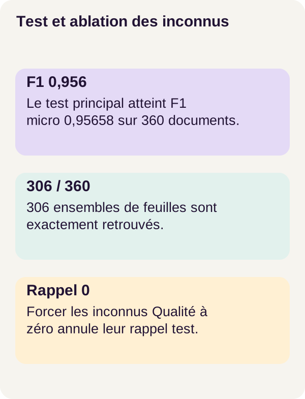
Exact-set counts offer another reading: 306 / 360 corresponds to 85% of documents with entirely correct leaves, versus approximately 54.17% for the complete node set. These percentages are calculated from published counts; they are not additional measurements.
Why can the two exactness measures differ? The network also produces parent scores. In an illustrative example, every leaf of a document may be correct, but the parent achats may be proposed unnecessarily. Closure does not remove this parent because it only propagates scores upward. The suggestion can therefore have no violations while including an unnecessary category.
This example shows a possibility of the mechanism. Aggregate figures alone cannot attribute every corpus error to this specific case: outputs must be examined document by document.
Examine difficult leaves and the simple reference
The two overall F1 scores are close, but this does not mean every leaf behaves the same. achats/factures is the weakest: its F1 is 0.82759, with 12 false negatives and 8 false positives. achats/fournisseurs scores 0.89320. qualite/audits reaches 0.90647 but has 13 false positives.
The Quality branch misses no expected leaf in the main test; nevertheless, it adds 17 false positives. Perfect recall can therefore coexist with wrongly suggested categories.
Finally, the lexical baseline scores 1.00 on this synthetic corpus with explicit patterns. It would be misleading to conclude that CamemBERT is necessary for these data. The tutorial studies learning with partial annotations and hierarchy; it demonstrates neither model superiority over this reference nor automatic transfer to a real DMS.
Exercise: predict the effect of hidden annotations
Formulate your hypothesis before running commands
We will mask 40% of known Quality-branch annotations in training, without changing validation or testing. These are document–label pairs, not 40% of texts removed, nor necessarily 40% of positive annotations alone.
Take a moment to predict the result. If this information becomes unknown, should we still penalize the model when it suggests a Quality leaf? What would happen if we wrongly told it that all these memberships were negative? Do you expect more omissions, more additions, or both?
The experiment compares two fresh models derived from the same initial model and using the same identifiers. exercise-correct removes unknown terms from the loss. exercise-wrong turns them into negative targets equal to zero. Each variant trains for three epochs.
This is not a change applied only to scores after training: the two models learn with different supervision. The workflow also checks that the main evaluation remains unchanged, so the exercise is not confused with the original r001 result.
docker compose run --rm learning python -m ged_classement_hierarchique.cli exercise --config configs/minimum.yaml
docker compose run --rm inference python -m ged_classement_hierarchique.cli predict --config configs/minimum.yaml --variant exercise-correct
docker compose run --rm inference python -m ged_classement_hierarchique.cli predict --config configs/minimum.yaml --variant exercise-wrong
docker compose run --rm tutorial python -m ged_classement_hierarchique.cli evaluate-exercise --config configs/minimum.yaml
Understand which way an incorrect target pushes the model
Return to an illustration independent of measurements: a probability score p = 0.8 for a category that is actually present. With correct target y = 1, BCE is -ln(0.8), approximately 0.2231. Replacing the target with y = 0 makes it -ln(0.2), approximately 1.6094. ln denotes the natural logarithm. The model is then heavily penalized for favoring a membership that is in fact real.
We can go one step further with the gradient: it indicates how loss changes when a score or parameter changes. For this BCE, the derivative with respect to the logit is p - y. With the correct target, it is -0.2; with the false negative target, it is 0.8.
If we reason in terms of directly adjusting this logit to reduce loss, the first case pushes it upward and the second downward. Updates in a shared network are more complex, but this example explains the direction of the erroneous signal. Masking the unknown target removes that signal; it does not reveal the missing truth.
Compare with observed results
The workflow's solution confirms that Quality logits decrease when unknowns become negatives. On the unchanged test set:
| Metric | Correct mask | Unknowns forced to zero |
|---|---|---|
| Quality leaf recall | 0.59149 | 0 |
| Quality false negatives | 96 | 235 |
| Macro F1 across all test leaves | 0.85430 | 0.65244 |
With the correct mask, the model finds 139 true positives, misses 96 memberships, and produces 92 false positives on Quality leaves. Recall follows directly: 139 / (139 + 96) = 139 / 235, approximately 0.59149.
The 235 expected Quality leaves here mean 235 positive document–leaf memberships, not 235 different categories or necessarily 235 distinct documents. Under the incorrect policy, all become false negatives: this branch's recall drops to zero.
Why does overall macro F1 remain at 0.65244 rather than zero? Because it covers all 12 leaves, not just Quality. Success on other categories can preserve a nonzero average while an entire branch is missed.
The correct mask also remains worse than the main model: macro F1 of 0.85430 versus 0.95619. It has lost supervised information. It avoids manufacturing negatives but does not recover hidden annotations. No increase in F1 was expected from this removal.
The lesson is precise: preserving the unknown protects the meaning of training data; it does not replace absent information.
Produce figures and clean up without losing evidence
Connect averages to examples
Generate figures from the results already calculated, then check educational milestones:
docker compose run --rm tutorial python lesson/figures/plot.py
docker compose run --rm tutorial python scripts/check_checkpoints.py
Figures represent existing results; they are not new experiments. The milestone check verifies educational material. Inspect the PNGs, outputs/evaluation.json, and outputs/exercise-comparison.json before deleting anything.
Also return to D-031: it explains the mechanism using a training example. Its readability does not replace measurements on the 360 separate documents. To judge classification, examine incorrect proposals as well as successful cases.
Clean only workflow outputs
Copy metrics and figures you want to preserve before these commands. The order below is part of the workflow: the first shutdown precedes cleanup; the last leaves the project stopped again after the cleanup container runs.
docker compose down
docker compose run --rm tutorial python scripts/clean.py --outputs-only
docker compose down
clean --outputs-only displays and removes only outputs. The corpus, model, and checkpoints are preserved. This targeted cleanup requires neither a global Docker purge nor removal of other projects' resources.
If something goes wrong
The GPU is visible on the host, but computation fails inside Docker? Return to the preflight and check_environment.py. The second check verifies actual access from the container; the first does not replace it.
A target is rejected or the loss is unusable? Check matching shapes, the mask's boolean type, and the values of known annotations only. Do not replace unknowns with zero to make the problem disappear. A zero count calls for handling an unsupervised batch, not forcing a mean calculation.
The hierarchy looks correct but classification is wrong? Examine added or missed leaves, extra parents, and per-category errors. No violations does not test content relevance. Also check that each column still corresponds to the same taxonomy node.
Move from prototype to useful application
Start with a versioned taxonomy, audited annotations, and separate evaluation by department, language, and document type. A new category or reorganized branch changes the classification contract: preserve the correspondence between data, outputs, and the plan's version.
For annotation, distinguish “yes,” “no,” and “not reviewed” in the interface. An empty box should not automatically become a negative example without an explicit rule. This is a product decision to design for an adaptation, not an interface already delivered by this prototype.
Show reviewers the proposed leaves and their ancestors. Plan what should happen with low scores and leaves the model never proposes. A confirmation button must not hide a missed category simply because the overall average looks good.
Hierarchical closure ensures compatibility with the plan; it certifies neither content relevance nor classification permissions. Access authorization and any action on the document remain separate decisions. The POC still moves no files and grants no rights.
We have learned to separate available text, known annotations, learned scores, hierarchical consistency, and measured correctness. This separation lets us understand an error and decide what to improve rather than rely on a single score.
Further references
Links to CamemBERT, the Transformers glossary, and PyTorch clarify encoding, masks, sigmoid, and loss. The scikit-learn references specify metric conventions; they do not claim that the project calls those functions. The article's small numerical examples explain operations and remain separate from Vesta corpus results.
To reproduce r001, retain the ZIP's files and versions. Online documentation can evolve; its generic examples do not replace the tutorial's validated configuration.
Download the r001 course: r001 ZIP.