Train shapes from noise, then verify them

Imagine a small graphics tool with three choices: disk, ring, and cross. You select “ring” and request a new image. Simply drawing that shape in a web application would take only a few geometric rules or an SVG. But how could a neural network learn to produce it starting from nothing but an image of noise?

That is this tutorial's question. We will create examples whose construction we know, train a small diffusion model, and examine what it actually learned. The supplied program is a command-line Python workflow, not a graphical interface: the three shapes provide an experimental setting.

The result deserves stating from the outset: the model learns to predict noise better, but this configuration produces no masks accepted by the project's geometric criteria. This is not a detail to hide behind a descending curve. It is precisely what teaches us to distinguish progressing training from a generator that meets the need.

Download the tutorial archive.

What we are building

We are building conditional diffusion on 32 × 32-pixel images. “Conditional” means the network receives extra information: the requested class, disk, ring, or cross. We do not send it a French description; here, the condition is a class identifier.

The images are masks: every pixel estimates what fraction of its area belongs to the shape. A fully exterior pixel is 0, a fully interior pixel is 1, and a pixel crossed by the boundary can have an intermediate value. There is one channel, not three red, green, and blue channels.

The workflow separates three operations. During training, we start with known masks, add known noise, and modify network parameters so it learns to predict that noise. During generation, we hold those parameters fixed and start from noise to gradually construct an image. During evaluation, rules external to the network check the outputs.

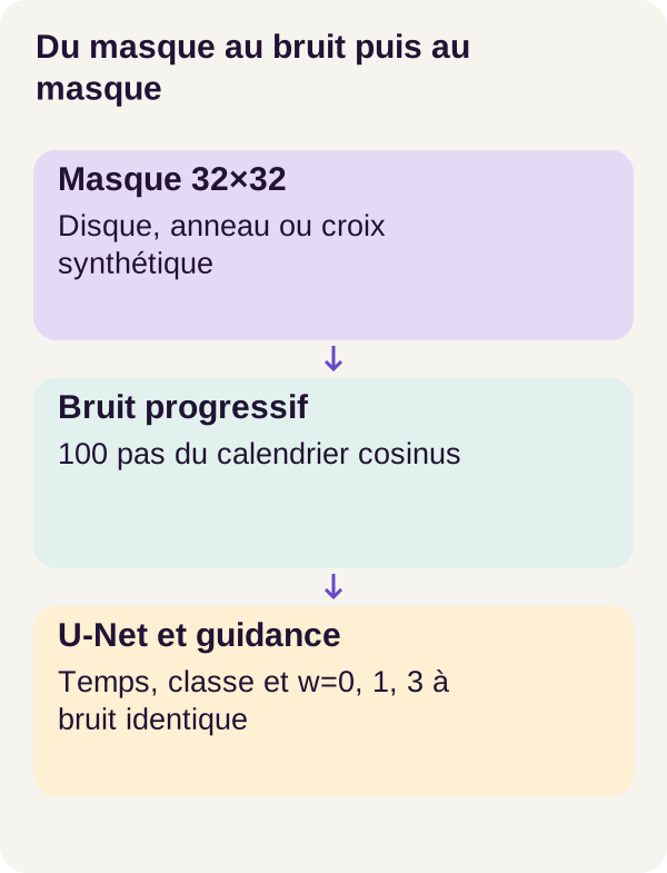
The network is a U-Net, whose role we will explain. It also learns to work without a specified class through a special condition called the null class. We can then compare its predictions with and without a shape indication and combine them using classifier-free guidance.

The case is deliberately synthetic: it produces neither photographs nor industrial drawings. Its value lies elsewhere. A ring must retain a hole; a disk must not turn into isolated pieces. These properties give us concrete questions to ask of results beyond “this image looks interesting.”

Concepts to keep in mind

A noisy image is still an array of numbers

A tensor is an array of numbers with one or more dimensions. For our mask, 1 × 32 × 32 means one channel, height 32, and width 32. An image batch adds a leading dimension: number of images, channels, height, width.

Gaussian noise is also an array, with one random value per pixel. “Gaussian” describes those values' distribution: they cluster around zero, with more small than extreme values. This noise is neither a file error nor a badly downloaded image. We deliberately add it and retain the sampled values so we know what the network should predict.

In network computations, clean pixels are mapped from [0, 1] to [-1, 1] with x * 2 - 1. Thus 0 becomes -1, 0.5 becomes 0, and 1 remains 1. Noise and noisy states are not bounded to that interval.

The forward path: adding a known difficulty

Forward diffusion transforms a clean mask, written x₀, into a noisy mask x_t. The index t indicates the selected diffusion level, not a duration in seconds.

The formula used is:

x_t = √ᾱ_t x₀ + √(1 − ᾱ_t) ε

You can read it without starting with a proof: some clean image plus some noise. ε, the Greek letter “epsilon,” denotes the sampled noise. ᾱ_t, “alpha bar at step t,” controls how much signal is retained. The square roots determine the coefficients actually applied.

Take an invented calculation on a single value, unrelated to measured model output. With x₀ = 1, ᾱₜ = 0.64, and ε = -0.5, we obtain:

xₜ = 0.8 × 1 + 0.6 × (-0.5) = 0.5.

The result is not obtained by erasing 36% of pixels. Every value is transformed by the mixture. Nor are the coefficients two opacities whose sum should be 1.

A noise schedule determines how these coefficients evolve. The project uses a 100-step cosine schedule. It is defined by the program, not learned with network weights. The cosine-schedule principle is presented in Improved Denoising Diffusion Probabilistic Models. This reference explains the schedule family without replacing the project's parameters.

What the network actually learns

During training, the network receives the noisy image, step t, and class. It must return estimated noise, not a finished disk or ring directly. We know the correct answer because we sampled noise ε ourselves.

The loss measures the difference between this prediction and the injected noise. Here it is MSE, mean squared error: compute differences, square them, then take their average.

A second educational example, limited to two values, is enough to follow the calculation. The actual noise is [0.2, -0.4], and the network predicts [0.1, -0.2]. Squared differences are 0.01 and 0.04, so MSE is (0.01 + 0.04) / 2 = 0.025. An error twice as large contributes four times as much to this loss.

Weights are the network's adjustable numbers. Gradients indicate how changes to these numbers affect loss; the optimizer uses them to update weights. We therefore do not code a “draw a ring” rule into the network: we adjust its weights from noisy examples and their expected answers.

Watch the two meanings of “step.” The 100 diffusion steps describe noise levels and the generation path. The 2,000 updates mentioned later describe weight training. They are not two ways of counting the same loop.

Why a U-Net?

The U-Net applies convolutions, learned filters that combine neighboring values. Its downsampling path reduces resolution to aggregate information; its upsampling path restores fine resolution. Connections between the paths reintroduce spatial detail. The U-Net authors' website presents this two-path architecture.

In src/mask_diffusion/unet.py, ConditionalUNet.forward() combines numerical time and class representations, then supplies them to network blocks. Time indicates the noise level at which it is working. Class indicates the requested mask family.

Its output has the same shape as the noisy image: a noise estimate for every pixel. The sampling program then uses that estimate to compute the next state. This distinction between the network and surrounding computation is central to DDPM.

A condition is not a guarantee

The null class means “no specified class.” It is neither a fourth shape to draw nor an instruction to produce an empty image. The same network must be able to supply conditional and unconditional estimates.

The principle of Classifier-Free Diffusion Guidance is to also learn without conditioning, removing it from some examples, then combine both estimates during generation. We need no separate classifier to calculate that combination. This obviously does not remove the need to evaluate images after producing them.

In this project, the combination is ε_u + w(ε_c − ε_u), where u denotes the unconditional prediction and c the conditional prediction. We will read it in the code: w=0 retains u, and w=1 retains c. A larger value is not a promise of a better image.

Docker and GPU prerequisites

You should be able to read Python functions, work with arrays, and run terminal commands. Docker basics are required; no prior knowledge of diffusion models is assumed.

The workflow requires Linux x86_64, Docker Compose, NVIDIA Container Toolkit, a 24 GiB RTX 3090, 16 GiB of RAM, and 16 GiB of available disk space, excluding shared Docker layers. These are the resources specified for this tutorial, not proof of compatibility with every hardware setup.

The GPU, or graphics card, runs network computations here using CUDA. A card visible to Linux may nevertheless be inaccessible to Docker. The supplied check therefore does more than list a device: it initializes CUDA inside the container and performs a computation. If needed, select the card before the workflow with export GPU_DEVICE=0, or with a card UUID, its unique identifier.

Computation is network-isolated. Containers use a read-only filesystem, no-new-privileges, dropped Linux capabilities, and CPU, RAM, and process-count limits. These restrictions bound execution; they do not prove image quality. Do not confuse isolated computation with fully offline installation either: building Docker images and acquiring dependencies may require network access.

A checkpoint is a saved state that can preserve or resume a computation. Locally produced Torch artifacts must remain trusted: do not load an arbitrary third-party checkpoint to replace a missing file. The torch.load documentation recalls loading precautions.

Data whose construction we know

Building a reference before asking the model to learn

Our experiment does not require collecting images from the Internet. We can define a disk, ring, and cross using geometric rules. The following function creates training examples; it is not the neural generator we will evaluate later.

It receives a label identifier, center, radius, thickness, and angle. Identifiers 0, 1, and 2 denote disk, ring, and cross respectively.

def render_mask(label, center=(0.0, 0.0), radius=0.55, thickness=0.18, angle=0.0):
    # Four subpixels in each direction; occupation fraction is the antialiased pixel.
    axis = (np.arange(128) + 0.5) / 64 - 1
    x, y = np.meshgrid(axis - center[0], axis - center[1])
    u = x * np.cos(angle) + y * np.sin(angle)
    v = -x * np.sin(angle) + y * np.cos(angle)
    distance = np.sqrt(x * x + y * y)
    if label == 0:
        inside = distance <= radius
    elif label == 1:
        inside = (distance <= radius) & (distance >= radius - thickness)
    elif label == 2:
        inside = ((abs(u) <= radius) & (abs(v) <= thickness / 2)) | (
            (abs(v) <= radius) & (abs(u) <= thickness / 2)
        )
    else:
        raise ValueError("Unknown geometric class")
    return inside.reshape(32, 4, 32, 4).mean((1, 3)).astype("float32")[None]

What did this function just do?

axis places the centers of 128 small intervals between -1 and 1. meshgrid constructs coordinates for a 128 × 128 grid. Subtracting center shifts the shape without changing its rules. Coordinates u and v apply the rotation used to construct the cross.

For a disk, each position is inside if its distance from the center does not exceed radius. For a ring, that distance must also be at least radius - thickness: the center stays empty. For a cross, the program combines two perpendicular rectangles. An unknown class identifier triggers an error rather than selecting a default shape.

Why a 128 × 128 grid when the output is 32 × 32? For anti-aliasing, which reduces stair-step effects at boundaries. Every final pixel is represented by four subpixels in each direction, or 16 subpixels. reshape(32, 4, 32, 4).mean((1, 3)) computes their mean occupancy.

For example, 12 interior subpixels out of 16 give 0.75. This gray is not an uncertain prediction: it represents an area fraction in our rendering method. Anti-aliasing therefore belongs to the data itself, not to retouching applied after evaluation.

Finally, astype("float32") selects 32-bit numerical storage. [None] adds the channel dimension. We obtain a 1 × 32 × 32 array, without a batch dimension at this stage.

Splitting data before training

Preparation produces three balanced sets. The following table spells out the project's counts; per-class counts follow from this balance.

Set	Number of masks	Masks per class	Role
Training	3,000	1,000	Supply examples used to modify weights.
Validation	600	200	Measure loss on examples separate from training.
Test	600	200	Keep a distinct set for the project's intended evaluation.

Each split uses a different seed for its pseudorandom draws. A seed initializes a generator; it is not an image annotation. Each image is also hashed, and any duplicate is rejected before the sets are frozen.

Hashing produces a content fingerprint. It detects identical content, not a guarantee that different shapes can never be very similar. In a small world of disks, rings, and crosses, that nuance matters. The null class does not add a fourth mask category to this table: it affects how the network is conditioned.

Core code: learning noise, then guiding the reverse path

Generating is not rerunning geometric drawing

The sampler starts from a noisy state and computes subsequent states in reverse diffusion order. Here, it calls the model twice at every step, combines the two predicted noises, and adds fresh Gaussian noise except at the last step.

It does not consult render_mask() to retrieve the expected shape. It must produce an image from what the network learned.

def guidance(unconditional, conditional, weight):
    return unconditional + weight * (conditional - unconditional)


def reverse_step(x, epsilon, t, schedule, noise):
    beta = schedule["beta"][t].to(x.device)
    alpha = schedule["alpha"][t].to(x.device)
    abar = schedule["abar"][t].to(x.device)
    previous = schedule["abar"][t - 1].to(x.device)
    mean = (x - beta * epsilon / (1 - abar).sqrt()) / alpha.sqrt()
    variance = beta * (1 - previous) / (1 - abar)
    return mean if t == 1 else mean + variance.sqrt() * noise


@torch.no_grad()
def ancestral_sample(
    model, initial, labels, weight, schedule, generator, start=None, stop=0
):
    x = initial.clone()
    trajectory = [x[0].cpu()]
    start = start or len(schedule["beta"]) - 1
    for t in range(start, stop, -1):
        times = torch.full((len(x),), t, device=x.device, dtype=torch.long)
        u = model(x, times, torch.full_like(labels, NULL_CLASS))
        c = model(x, times, labels)
        eps = guidance(u, c, weight)
        noise = (
            torch.randn(x.shape, device=x.device, generator=generator)
            if t > 1
            else torch.zeros_like(x)
        )
        x = reverse_step(x, eps, t, schedule, noise)
        trajectory.append(x[0].cpu())
    assert torch.isfinite(x).all()
    return x, torch.stack(trajectory)

Reading guidance with three numbers

The first function applies exactly the stated formula: unconditional + weight * (conditional - unconditional).

Let us take a fictional arithmetic example with a single noise value, with u = 0.2 and c = 0.5. These are not outputs captured from the model.

Project weight	Calculation	Result	Meaning of the operation
w=0	0.2 + 0 × (0.5 - 0.2)	0.2	Keep the unconditional prediction.
w=1	0.2 + 1 × (0.5 - 0.2)	0.5	Keep the conditional prediction.
w=3	0.2 + 3 × (0.5 - 0.2)	1.1	Extend the difference beyond the conditional prediction.

w=3 is an extrapolation, not a 75% / 25% mixture. The value 1.1 does not mean “110% confidence”: we are manipulating a noise estimate, not a probability. If the two branches return exactly the same estimate, their difference is zero and changing w does not change this combination.

A notation trap in the references. Ho and Salimans’ paper writes the combination as (1 + w_article) × c - w_article × u. Our code’s convention is w_projet = 1 + w_article. Keep the project’s values and formula together: w=0 in this tutorial does refer to the unconditional branch, whereas w=0 in the paper’s formula refers to the conditional branch.

Reading a reverse step without losing the thread

reverse_step() receives the current state x, the predicted noise epsilon, and the step number. The schedule provides beta, alpha, and abar. In this diffusion notation, alpha is 1 - beta and abar is the product of the alpha values up to the current step. previous retrieves the cumulative value at the preceding step.

The mean = ... line corrects the state from the predicted noise and the schedule coefficients. The variance = ... line sets the magnitude of the random noise used to draw the next state. The predicted noise epsilon and the newly drawn noise noise therefore do not have the same role. The first comes from the network; the second retains a random stage in this sampler.

The function returns this new noise for t > 1. At t == 1, it returns only mean. Adding noise during the return may seem paradoxical, but the program is not unrolling the exact history of one particular image backward: it constructs a generation trajectory according to the sampling rule.

Following the loop and what it retains

initial.clone() creates a working state without overwriting the array supplied by the caller. At every step, times contains the same index t for every image in the batch. The calls u = model(...) and c = model(...) use the same network, first with a null class and then with the requested classes.

In this excerpt, both calls take place even for w=0 or w=1: the code has no shortcut for these values. For a full 100-step trajectory, this amounts to 200 calls to the network per batch, not 200 weight updates.

The @torch.no_grad() decorator disables gradient tracking during this generation. There is no training-loss calculation or optimizer update here. That decorator does not replace a possible model.eval(), however: PyTorch distinguishes evaluation mode from gradient tracking. The excerpt does not show how the caller prepares the network mode.

Also note trajectory.append(x[0].cpu()). The trajectory retains only the first image in the batch, on the CPU. The final value x, by contrast, contains all images in the batch. With a start at 100 and stop=0, the loop processes 100, 99, …, 1, and the trajectory contains the initial state plus the 100 computed states: 101 states in total.

The final assertion torch.isfinite(x).all() requires finite numeric values: neither NaN nor infinity. It verifies neither contours nor holes, nor even that values stay within [0, 1]. An array that is numerically valid is not yet a valid shape.

Same initial noise: necessary, but not the whole story

The protocol compares w=0, w=1, and w=3 with identical initial noise. This is essential so that a difference created at the start is not attributed to the guidance weight.

But the loop also draws new noise using generator. To fully isolate the effect of w in a paired comparison, the same sequence of intermediate draws must also be reproduced. The sampler receives this generator; it does not reset it itself. Two successive calls with the same generator object may therefore consume two different portions of its sequence.

This detail follows from the displayed code: retaining initial alone is not enough to establish control over every draw. Initializing and saving the generator belong to the caller code in the complete project.

The same question arises on resumption. With start=100 and stop=50, the loop processes steps 100 through 51 and returns the state at level 50. Resuming from that state with start=50 also requires recovering the corresponding random state, along with the same model and schedule. The PyTorch reproducibility documentation explains why setting a seed alone does not guarantee identical results across all environments.

Measuring learning with a fixed validation exercise

During training, the program draws a time, adds ε, and minimizes the error in predicting ε. To compare two network states, the following validation instead uses times and noises fixed in advance. This is equivalent to using the same test data after every change to an application.

def validation_mse(model, config):
    assert (
        sha("outputs/validation-noise.npz")
        == read_json("outputs/validation-lock.json")["sha256"]
    )
    data = np.load("outputs/validation.npz")
    fixed = np.load("outputs/validation-noise.npz")
    total = 0.0
    model.eval()
    with torch.no_grad():
        for i in range(0, 600, 64):
            x = torch.from_numpy(data["images"][i : i + 64]).cuda() * 2 - 1
            t = torch.from_numpy(fixed["times"][i : i + 64]).cuda()
            eps = torch.from_numpy(fixed["noise"][i : i + 64]).cuda()
            y = torch.from_numpy(data["labels"][i : i + 64]).cuda()
            noisy = sample_noisy_image(
                x, t, eps, cosine_schedule(config["diffusion_steps"])
            )
            total += float((model(noisy, t, y) - eps).square().double().sum())
    model.train()
    return total / (600 * 32 * 32)

The initial assertion compares the SHA-256 fingerprint of outputs/validation-noise.npz with the one recorded in outputs/validation-lock.json. It checks this fixed noise file; it is not a universal verification of every project file.

The program then loads the 600 validation images, times, noises, and classes. .cuda() places the arrays on the GPU. The * 2 - 1 transformation applies the mask rescaling explained above.

model.eval() enables evaluation mode, while torch.no_grad() disables gradient tracking. Then sample_noisy_image() creates each noisy input. We compare model(noisy, t, y) with eps, not with the clean image x: the score still concerns noise.

The loop advances in batches of 64. With 600 images, that gives nine full batches and a final batch of 24. The code adds the squared errors, then divides by 600 × 32 × 32 = 614 400 pixel values. It does not average batch averages, which would give too much weight to the smaller last batch.

.double() converts the squared errors before their sum; it does not turn the whole network into a model that computes in double precision. Finally, model.train() returns the network to training mode.

The constants 600, 32, and 32 belong to the protocol. If you change the validation or image size in another experiment, this calculation must change with the data. Keep them unchanged in the reference path.

Set up and verify the environment

Extract the archive, then open a terminal at its root. Every command that follows starts from this same directory. Use an extraction dedicated to the experiment so you do not mix its files with those of another project.

Start by preparing the directories, checking Compose, building the images, and testing the environment:

sh scripts/setup.sh
docker compose config --quiet
docker compose build acquire gpu
docker compose run --rm acquire python scripts/acquire.py --config configs/minimum.yaml
docker compose run --rm gpu python scripts/check_environment.py --config configs/minimum.yaml
docker compose run --rm gpu python -m pytest -q

setup.sh prepares the project. docker compose config --quiet checks the Compose configuration without displaying it; no output alone is therefore not an anomaly. build acquire gpu builds the two named services.

acquire checks the project locks. No pretrained model is downloaded in this tutorial: masks will be generated by prepare, and the network will be trained in the learning path. Do not transplant the weight-acquisition stage from a language-model tutorial here.

check_environment.py must confirm that the GPU is genuinely usable from the container. The pytest command then runs the project tests. Fix every error before training; generation results could not repair a missing environment check.

Now prepare the images, then inspect their transformation by noise:

docker compose run --rm gpu python -m mask_diffusion.cli prepare --config configs/minimum.yaml
docker compose run --rm gpu python -m mask_diffusion.cli inspect-noise --config configs/minimum.yaml

After prepare, the stated datasets are 3,000 training masks, 600 validation masks, and 600 test masks. inspect-noise lets you observe the forward path. At this point, see how a known shape becomes a noisy state; you are not yet observing the model’s ability to generate a shape.

Train, resume, and evaluate

Run the reference path

We first verify the U-Net dimensions and gradients, then train the model. Gradients are useful here to check that the computation can actually change its parameters; seeing an output image would not establish that.

The sequence also includes a deliberate interruption and resumption. A complete reference training run is used to compare an interrupted, then resumed, training run. This is therefore not an instruction to manually interrupt the first command.

docker compose run --rm gpu python -m mask_diffusion.cli inspect-model --config configs/minimum.yaml
docker compose run --rm gpu python -m mask_diffusion.cli train --config configs/minimum.yaml
docker compose run --rm gpu python -m mask_diffusion.cli train --config configs/minimum.yaml --stop-after 1000 --run-name interrupted
docker compose run --rm gpu python -m mask_diffusion.cli train --config configs/minimum.yaml --resume artifacts/checkpoints/interrupted/state.pt --run-name resumed
docker compose run --rm gpu python -m mask_diffusion.cli compare-resume --config configs/minimum.yaml
docker compose run --rm gpu python -m mask_diffusion.cli sample --config configs/minimum.yaml
docker compose run --rm gpu python -m mask_diffusion.cli evaluate --config configs/minimum.yaml

inspect-model comes before lengthy calculations. The first train produces the reference training. The call with --stop-after 1000 --run-name interrupted creates the interrupted branch. The next call resumes its checkpoint artifacts/checkpoints/interrupted/state.pt under the name resumed. compare-resume compares the resulting states.

sample then uses the models to produce outputs, and evaluate applies the measurements. The figures presented below are those from the validated reader reproduction of revision r1. They are not thresholds to reach by changing settings until a pretty image appears.

Define what each measurement can tell us

The validation MSE compares predicted noise to fixed reference noise. It answers, “does the network predict noise better in this exercise?” It does not directly answer, “does the request for a ring produce a ring?”

Geometric compliance examines produced images with rules separate from the network. The project uses component, hole, and area checks. A component is a connected region; a hole is a background region enclosed by a shape; area measures its extent according to the validator’s rule.

To visualize these notions, think about ideal shapes, not an exhaustive description of the project’s classifier. A disk is filled, a ring has a hole, and a cross has arms. The number of holes alone is not enough to tell a cross from a disk. Exact decisions depend on the validator’s rules, especially how it interprets intermediate pixels. Thresholds are not detailed in this article’s excerpts: read them in the archive’s evaluation code rather than inventing new ones.

The unknown category means none of the three geometric classes was assigned. It is not a fourth success. An image that looks vaguely circular to the eye may therefore remain rejected by the chosen criteria.

Distance to train, meaning the training set, is the MSE between an output and its closest training mask. Here, we compare images with each other; this is not noise-prediction MSE. A small distance indicates strong closeness under this measurement, but does not by itself prove memorization. Conversely, a large distance does not prove interesting creation: shapeless noise can be very far from the examples.

Finally, diversity concerns the variety of outputs. It must be read together with compliance and proximity to the training data. Three hundred different outputs that are all invalid do not make a usable generator of varied shapes. This article provides no numerical diversity or distance-to-train value, so we will not draw a conclusion about memorization.

Observed results

Training and resumption work in the measured path

The main training run performed 2,000 updates and processed 128,000 examples with repeated images from the training set. These are not 128,000 distinct masks: the same clean images can be presented several times, with drawn training times and noises.

Validation MSE fell from 1.1551 to 0.0211. The network therefore improved on the task that was actually measured: predicting validation noise.

Two checks concern resumption. After training stopped at step 1,000, resumption recovered the same parameters, with a maximum error of zero. The sampler resumed at t=50 also gave a maximum error of zero. These equalities concern comparisons made in this path; they do not promise bit-for-bit identity on all hardware or software versions.

But no run produces a compliant mask

The protocol crosses two network states, untrained and trained, with three guidance weights. This yields six runs of 300 samples each. The table expands this distribution without adding new measurements:

Network state	Guidance	Geometric compliance	Outputs classified unknown
Untrained	w=0	0/300	300
Untrained	w=1	0/300	300
Untrained	w=3	0/300	300
Trained	w=0	0/300	300
Trained	w=1	0/300	300
Trained	w=3	0/300	300

“Untrained” and “unconditional” do not mean the same thing. The former describes the state of the weights; the latter describes the absence of a class during a prediction. The trained network can therefore be used in the unconditional branch with w=0.

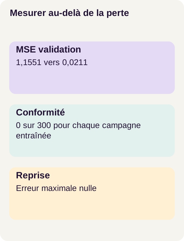
The 300 outputs from every run were all classified as unknown. The lower MSE is therefore not evidence that generations respect the requested shape. It would be misleading to present only the loss curve, or to select a few visually favorable images to claim a successful generator.

What we learned

A good answer to a subtask is not yet a good final result

For a web developer, the analogy is a function whose unit tests improve while the complete user journey still fails. The two observations do not contradict each other: they concern different levels of the system.

Here, loss measures an average of numerical errors on noise. Generation chains calculation steps; final evaluation requires a shape whose properties are accepted. These three objects must remain distinct.

As an illustration, not a diagnosis of this experiment, a small break in the edge of a ring can change whether its hole exists. A few pixels can therefore flip a geometric criterion while the average error changes little. This helps explain why a score for a numerical task does not automatically become geometric compliance.

Reproducing a failure is still useful information

The diffusion mechanism, guidance identities, and preservation of resumption state are verified in the reported path. At the same time, the geometric rules show a clear limit: this configuration does not produce the desired compliant small masks.

An identical resumption shows that the calculation could continue coherently under the test conditions. It does not show that the result is good. Likewise, a higher guidance weight does not automatically fix inadequate generation.

The aggregated measurements do not allow the failure to be attributed to one single cause. Saying “it is enough to train longer” or “the validator is necessarily too strict” would go beyond what has been established. These are possible hypotheses to examine separately with their own checks, not already validated fixes.

Exercise: state the hypothesis before the command

Before running anything, calculate guidance(u, c, 0) and guidance(u, c, 1) with values of your choice. Also check what happens when u and c are equal: can the weight still change the combination?

Then state a hypothesis: when moving from w=1 to w=3, with identical initial noise, will diversity remain, decrease, or shift? Note what is algebraic certainty, such as the identities at weights 0 and 1, and what is a prediction about the network’s outputs.

Now run the provided exercise:

docker compose run --rm gpu python -m mask_diffusion.cli exercise --config configs/exercise.yaml

The output checks the limiting identities, retains the same initial noise, and reports the metrics for w=1 and w=3. It does not promise any improvement.

Compare these observations with your hypothesis. To interpret a difference as an effect of weight alone, also consider the state of the intermediate-noise generator, not only the starting noise. Finally, do not replace “more visible variations” with “more valid shapes”: useful diversity must meet the task’s criteria.

Adapt and produce

Before turning this experiment into an application, its generation limitation must first be addressed. Adding an API around the model would not make the masks more compliant.

A further experiment, separate from r1, could examine one hypothesis at a time: for example, study the effect of training duration while retaining the data, schedule, and validator. It would need to retain the reference outputs, document the change, and measure noise, compliance, and diversity again. No result from this variant is stated here. Changing acceptance rules after seeing the images would define another task, not a demonstrated improvement of the old model.

For real use, the synthetic masks would need to be replaced with authorized, versioned data, with annotations and explicit business criteria. Failures would need to be measured across relevant populations: image type, class, or acquisition condition, depending on the need. It would also be necessary to track drift, meaning changes in data or results after deployment.

Rights management, authentication, API protection, observability, backups, load, and a rejection policy still need to be built. A stable loss covers none of these requirements. The tutorial provides a measurable experiment, not a service ready to receive business images.

Troubleshooting and cleanup

If the GPU check fails, check the driver and the NVIDIA Container Toolkit installation, then run check_environment.py again with the command shown above. A card visible on the host but inaccessible in the container first indicates a Docker/GPU integration issue, not a reason to modify the U-Net.

If a file or checkpoint check fails, keep its message and verify that the files belong to the same run and configuration. Do not bypass an integrity failure with an unidentified external checkpoint.

If loss falls while compliance remains at zero, you have not necessarily run the program incorrectly: that is precisely the limit observed in this revision. Examine states and measurements without turning an expectation of success into a stated result.

To produce figures, check checkpoints, preview cleanup, then stop services, use the path’s commands:

docker compose run --rm gpu python lesson/figures/plot.py
docker compose run --rm gpu python scripts/check_checkpoints.py
docker compose run --rm gpu python scripts/clean.py --scope generated --dry-run
docker compose down --remove-orphans

plot.py produces the figures; it is not another training run. check_checkpoints.py checks the checkpoints. The --dry-run option means cleanup is only previewed: it does not delete generated files.

Finally, docker compose down --remove-orphans stops and removes the resources concerned by the Compose project. Local files are retained in this path. There is no need to perform a global Docker purge, which would affect other experiments.

Primary sources and documentation

The results in this article are those of the r1 reproduction of the downloadable project. The following references can be used to explore the mechanisms and precautions further; they do not independently validate its outputs.

Diffusion and architecture. Ho, Jain, and Abbeel — Denoising Diffusion Probabilistic Models describes the DDPM framework. Ho and Salimans — Classifier-Free Diffusion Guidance presents the combination of predictions with and without a condition; note the weight convention explained above. Nichol and Dhariwal — Improved Denoising Diffusion Probabilistic Models presents, among other things, the cosine schedule. The U-Net authors’ website explains the original architecture.

Computation and resumption. PyTorch documentation distinguishes evaluation mode and gradient tracking, explains the limits of reproducibility, and documents loading with torch.load. These general pages do not replace the versions and settings retained in the archive.

Environment. The Docker Compose GPU support documentation and the NVIDIA Container Toolkit installation guide detail access to the card from containers.

Download the archive and follow the complete path: open the tutorial.