





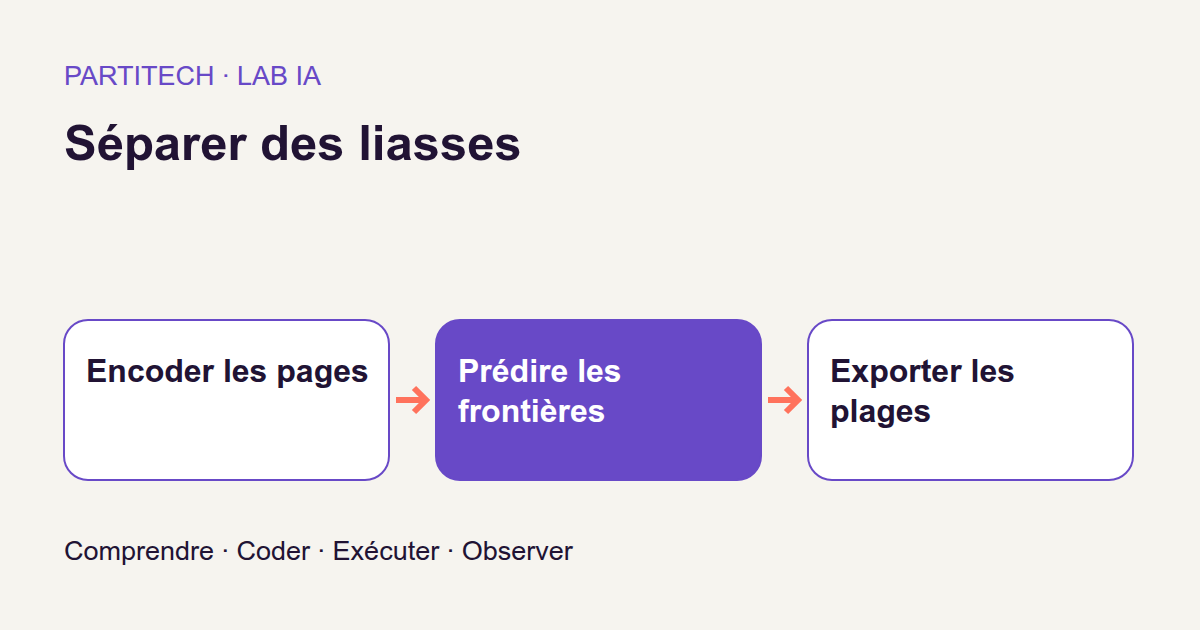
You are adding document import to a back office. A user uploads a single PDF, but the file actually contains several items to file separately: an invoice, another invoice, then a report. Where should you split it?
The first idea seems simple: detect changes in type. But two consecutive invoices remain two invoices, even when they concern different cases. Another idea: split when page numbering restarts at 1. This is a useful clue, but we will measure why it is not always enough.
This tutorial builds a pipeline that estimates whether a boundary exists between two neighboring pages, then assembles these decisions into complete documents. We work with fictional “Atlas” bundles. The goal is to understand and reproduce the mechanism, not deliver a filing service for real documents.
Download the r002 tutorial ZIP
For a nine-page bundle, the result might be a sequence of ranges: [0, 3], [3, 5], [5, 9]. Each range produces a separate PDF. Note the convention: the start is included and the end excluded, as in a Python array slice pages[start:end].
| Range | Indices of retained pages | Pages for the reader |
|---|---|---|
[0, 3] |
0, 1, 2 | 1 to 3 |
[3, 5] |
3, 4 | 4 to 5 |
[5, 9] |
5, 6, 7, 8 | 6 to 9 |
The page at index 3 is therefore not duplicated: it belongs only to the second range. This example illustrates the output format without describing a new corpus run.
Our goal has two distinct requirements: find the correct splits, then export the correct pages in order and without loss. A faithful export can contain a wrong split; correct segmentation does not guarantee preservation of every PDF property.
Useful concepts before running the model
A small binary question rather than business classification
A bundle here is a file containing several consecutive documents. Between any two pages, we ask the same question: “Does the next page start a new document?” The expected answer is 1 for a boundary and 0 for continuation. This is binary classification: there are only two possibilities.
A bundle of n pages has n - 1 internal split positions. Four pages therefore yield three decisions. The beginning and end of the file are already known: there is no need to ask the model whether a page exists before the first or after the last.
Missing a real boundary causes a merge: two documents remain in the same PDF. Adding a false boundary causes over-segmentation: one document is spread across multiple files. These errors differ, and we will count them separately.
The model does not learn to say “this is a valid invoice.” It learns to propose a separation. Identifying an item's type, case, or status afterward would be another task.
Turn page text into numbers
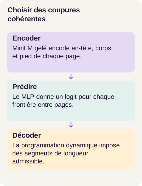
MiniLM acts as a text encoder here. It does not write an answer: it turns text into vectors, meaning lists of numbers the classifier can use. These representations are also called embeddings.
The workflow separately encodes each page's header, body, and footer. This preserves a distinction between regions rather than immediately mixing them into one representation. Observable geometry measurements then complement the text information.
Before encoding, the tokenizer splits text into units called tokens. A token may be a word, word fragment, or symbol; it is not necessarily a whole word. Special tokens also delimit the sequence. MiniLM produces a representation for each position.
A practical difficulty remains: two texts need not contain the same number of tokens. To process them together, the shorter one can be extended with padding. These positions support batch computation, not page description.
The attention mask distinguishes retained positions from padding. Masked pooling then averages the retained vectors to obtain a fixed-size representation. The Sentence Transformers pooling documentation describes this transition from a variable-length sequence to a fixed-size vector.
Consider a small illustrative calculation using two-dimensional vectors that do not come from MiniLM. Two valid positions are [2, 4] and [4, 2]; a padding position is [100, 100]. With mask [1, 1, 0], the mean is [3, 3]. Without the mask, it would be approximately [35.33 ; 35.33]: padding would completely distort the representation.
Its contribution must therefore be removed and the result divided by the number of valid positions, not by the padded array length. The official masked pooling code shows both operations.
What learns and what stays fixed
MiniLM's weights are frozen: they are not modified during this training. The encoder must still perform calculations to represent pages; “frozen” does not mean “computationally free.”
Only the MLP head, short for multilayer perceptron, is trained. Think of it as a small numerical function with adjustable parameters: it receives features from both pages and produces a boundary score. Its parameters are learned numbers, distinct from features, which are the numbers supplied as input.
During training, a loss function measures the gap between model output and the expected answer. BCE, or binary cross-entropy, penalizes high confidence on the wrong side. For a real boundary, predicting a probability of 0.9 incurs a penalty of -ln(0.9), approximately 0.1054; predicting 0.1 incurs approximately 2.3026. These values explain the calculation; they are not losses measured on Atlas.
The project uses PyTorch and BCEWithLogitsLoss, which receives raw scores directly and combines the operations in a numerically stable way. We will explain these scores, or logits, before reading the decoder.
Three methods, three roles to compare
The first method is a baseline, a simple reference point: split when the visible page number resets to 1. It is not a document-type classifier.
The second uses the MLP followed by a threshold: each split position is decided separately from its probability.
The third reuses MLP scores but chooses a complete partition under a maximum document length. It uses dynamic programming, which we will read as a search for solutions that reuses intermediate results.
The methods are compared on the same test set. Annotations, also called labels or gold, are reference answers. They serve training or measurement depending on their split; they are not observable page features. Test labels are never mounted in the inference and learning containers.
Training adjusts parameters, validation chooses the threshold, and testing measures the resulting rule. Length constraints are also declared before testing. Tuning these choices after looking at test answers would be like preparing a solution with the answer key open.
Prerequisites and environment checks
You need to be able to read Python, use a terminal, and run Docker. PyTorch handles training; NumPy is used notably in the decoder. The binary classification concepts are those we have just introduced.
The reference workflow is designed for Linux with a GPU. An RTX 3090 with 24 GiB, 24 GiB of RAM, and 25 GiB of disk space are recommended. VRAM is the graphics card's memory; RAM is the machine's memory. The r002 workflow actually used an RTX 3090, but these guidelines are not guaranteed minimums for every configuration. The results presented here establish no equivalent CPU workflow.
Unzip the archive and open a terminal at its root. All following commands run from this directory in the stated order. The project's versions and pinned files are the reference to reproduce; linked documentation helps explain mechanisms, not replace dependencies.
A GPU visible through nvidia-smi on the host is not necessarily usable in Docker. NVIDIA Container Toolkit provides the necessary integration with the container engine. The workflow's diagnostics report its absence and the required action without installing it for you. The GPU_DEVICE=1 variable can select another card before starting the workflow, depending on the supplied configuration.
Check the host and build services
sh scripts/preflight.sh
sh scripts/setup.sh
docker compose config --quiet
docker compose build acquisition tutorial inference learning
The preflight is the preliminary check: Docker, Compose, memory, disk space, and GPU visibility under Linux. The setup script then runs, after which Compose checks the configuration and builds the four services.
docker compose config --quiet succeeds without displaying a valid configuration; this is the documented behavior of the --quiet option. No output is not a reason to ignore an error exit code.
Acquire MiniLM and actually compute inside Docker
docker compose run --rm acquisition python scripts/acquire.py --config configs/minimum.yaml
docker compose run --rm tutorial python scripts/check_environment.py
docker compose run --rm tutorial python -m pytest -q
Acquisition downloads the MiniLM files, then compares their size and SHA-256 fingerprint with expected values. This fingerprint identifies file contents. Atomic replacement prevents a partially acquired file from being installed instead of the expected resource. No weights are included in the ZIP.
check_environment.py goes beyond the host check: it actually loads MiniLM in Docker and computes on the GPU. Finally, tests check dynamic programming, exports, and the length constraint among other things. The reference workflow reports 35 passing tests; passing them does not mean every real bundle will be correctly separated.
Produce boundary decisions
Prepare documents without giving their answers to the encoder
docker compose run --rm tutorial python -m pdfbundles.cli prepare --config configs/minimum.yaml
docker compose run --rm inference python -m pdfbundles.cli features --config configs/minimum.yaml
prepare generates fictional bundles and separates their annotations. features builds adjacent-page features in the container that cannot see those labels. Training will later use authorized supervision, but gold test splits remain reserved for evaluation.
For a pair of pages, the r002 report indicates a vector of 3,480 values supplied to the MLP and 462,209 trainable parameters in the head. The first number describes the input; the second describes the learned function. Do not confuse them with page or document counts.
These dimensions apply to the ZIP's configuration. The name “MiniLM” alone cannot reconstruct the exact feature assembly: to modify it, follow feature construction in the project rather than inventing extra columns from the total.
Train, interrupt, resume
docker compose run --rm learning python -m pdfbundles.cli train --config configs/minimum.yaml --mode interrupt
docker compose run --rm learning python -m pdfbundles.cli train --mode continuous --config configs/minimum.yaml
docker compose run --rm learning python -m pdfbundles.cli train --mode resume --config configs/minimum.yaml
docker compose run --rm learning python -m pdfbundles.cli verify-resume --config configs/minimum.yaml
An epoch is one pass over the training examples. The total budget here is fifteen epochs. The interrupt mode creates an interrupted run; continuous provides a control trained without that interruption; resume resumes the interrupted calculation. This does not mean training the same model three times in succession to accumulate forty-five epochs.
A checkpoint is a saved state for continuing or checking computation. verify-resume compares the resulting states to verify that interruption and resumption recover the continuous run's result.
This is a reproducibility check, not a document-quality measure. Two runs can reproduce exactly the same errors. The observed identity also applies to this environment: the PyTorch reproducibility documentation notes that changing platforms or versions can change results.
Choose the threshold on validation data
docker compose run --rm learning python -m pdfbundles.cli calibrate --config configs/minimum.yaml
calibrate selects the threshold using the validation set. A lower threshold may trigger more splits; a higher threshold may miss more. Evaluation must measure this trade-off rather than assume one choice is always preferable.
The workflow selects 0.5. Here, the command name calibrate describes choosing this decision rule. It does not prove that all probabilities reported by the model correspond to error frequencies in a real application.
From local logits to complete documents
Read a logit before making a decision
A logit is a raw number that can be negative or positive. The sigmoid function converts it into a boundary probability: p = 1 / (1 + exp(-logit)). Its definition appears in the PyTorch Sigmoid documentation.
| Illustrative logit | Approximate probability | Tendency at threshold 0.5 |
|---|---|---|
| -2 | 0.1192 | Continue the document |
| 0 | 0.5000 | Tie resolved according to convention |
| 3 | 0.9526 | Split |
At threshold 0.5, a strictly positive logit therefore favors a boundary and a strictly negative logit favors continuation. A score of 3 does not mean “three boundaries” or “three pages.”
Independent thresholding handles each position separately. That is enough to produce consecutive ranges, but imposes no maximum length on them. Dynamic programming adds precisely this constraint.
Score an entire partition
To evaluate a segmentation, the program selects one contribution at each internal position: log(p) if it splits, log(1 - p) if it keeps the pages together. It then sums these contributions.
Why logarithms? Multiplying many probabilities can produce tiny numbers. Adding their logarithms preserves the ranking of products while simplifying computation. The resulting score is negative or zero; the largest is best, even when all are negative. A score of -0.5 is therefore preferable to -3.
This score is a comparison criterion built from MLP outputs. It is not a calibrated probability that the entire bundle is perfectly separated. The decoder consults no annotations to calculate it.
The complete decoder code
The following function receives logits for internal positions and the maximum length. np denotes NumPy; score_segments and boundaries_of are helpers in the complete project. This block alone is neither a PDF reader nor an exporter.
def decode(logits, maximum):
    logits = np.asarray(logits, dtype=np.float64)
    if (
        logits.ndim != 1
        or not np.isfinite(logits).all()
        or not isinstance(maximum, int)
        or maximum < 1
    ):
        raise ValueError("Invalid logits or length constraint")
    n = len(logits) + 1
    boundary = -np.logaddexp(0, -logits)
    within = -np.logaddexp(0, logits)
    prefix = np.concatenate([[0.0], np.cumsum(within)])
    best = np.full(n + 1, -np.inf)
    previous = np.full(n + 1, -1, dtype=int)
    best[0] = 0
    for end in range(1, n + 1):
        candidates = []
        for start in range(max(0, end - maximum), end):
            # Internal non-boundaries are start..end-2, then one boundary at
            # end-1 unless this is the final segment of the whole bundle.
            segment = (
                prefix[end - 1]
                - prefix[start]
                + (boundary[end - 1] if end < n else 0.0)
            )
            candidates.append((best[start] + segment, -start, start))
        value, _, start = max(candidates)
        best[end] = value
        previous[end] = start
    segments = []
    end = n
    while end:
        start = int(previous[end])
        segments.append([start, end])
        end = start
    segments.reverse()
    direct = score_segments(logits, segments)
    if abs(direct - float(best[n])) > 1e-8:
        raise ValueError("Boundary counted more than once")
    return {
        "segments": segments,
        "boundaries": boundaries_of(segments),
        "score": direct,
        "maximum": maximum,
    }
We will follow the four important operations: validate input, score a segment, remember the best path, then reconstruct the ranges.
1. Validate input and establish the right indices
np.asarray(..., dtype=np.float64) prepares a double-precision numerical array. The function rejects arrays that are not one-dimensional, non-finite values such as NaN or infinity, and a length that fails the positive-integer check.
Python has a subtlety: isinstance(True, int) is true because bool is a subtype of int. The snippet therefore accepts maximum=True as a limit of 1. This check must not be presented as strict API parameter validation; that would need to be added at a real application's interface without silently changing the reference workflow.
The page count is derived from n = len(logits) + 1. Three logits describe four pages. Under this convention, an empty logit array describes a one-page bundle; it does not let the function identify a genuinely empty PDF. Source-document validation belongs to another step.
Ranges must respect three invariants, properties that always hold: start at 0, finish at n, and meet without gaps or overlaps. They must also be nonempty and no longer than maximum.
2. Calculate scores without counting a boundary twice
The boundary and within arrays contain log(p) and log(1 - p) respectively. They use np.logaddexp, which computes log(exp(a) + exp(b)) in a way suited to these numerical operations. The code thus works directly from logits without first rounding a sigmoid toward 0 or 1 and then taking its logarithm.
For a segment [start, end], pages run from start to end - 1. Continuations within the segment are therefore at indices start through end - 2.
Take [0, 3]: it contains pages 0, 1, and 2. We keep 0–1 and 1–2 together. If more pages follow, we add a split between 2 and 3. If 2 is the file's last page, that outgoing split does not exist.
That is exactly the role of boundary[end - 1] if end < n else 0.0. The end of the file adds no artificial internal boundary.
The prefix array contains cumulative sums of within. Adding a segment's continuations therefore requires only one subtraction: prefix[end - 1] - prefix[start]. This is the same principle as a running total used to calculate a subtotal between two positions without repeating the entire sum.
The boundary before a segment has already been counted by the previous segment. The new segment counts its continuations and, if present, its outgoing boundary. This division of responsibility prevents double counting.
3. Keep the best result for each possible ending
Dynamic programming here rests on one question: “To end a segment at this page, which start gives the best total score?”
best[end] stores the best score for the first end pages. An important detail in this implementation: when end < n, this score already includes the outgoing split after those pages. previous[end] stores the start of the last selected segment.
best[0] = 0 initializes the path before any page. Other scores start at negative infinity so a state not yet reached cannot win a comparison.
For an ending end, the loop explores all starts from max(0, end - maximum) to end - 1. This allows segments of 1 to maximum pages. Each candidate adds the best known prefix score to the new segment's score.
Why is one best score per position enough? In this code, the next segment's score depends only on its boundaries and the logits it uses. It does not need to know the type or number of preceding documents. Reusing the best prefix therefore excludes no better possible continuation under this criterion.
For exactly equal scores, the tuple (score, -start, start) breaks ties. Python compares tuples element by element: max therefore prefers the smallest start, hence the longest current segment. This is a deterministic convention, not information about the document's nature. It does not mean the code explicitly minimizes the total number of documents.
4. Return from the score to the ranges
Once the final position is reached, while end follows predecessors backward. The last range is found first, then the second-to-last, and so on. segments.reverse() restores reading order.
The score of the reconstructed ranges is then recalculated by score_segments. A difference greater than 1e-8 from the dynamic score triggers an error. This check detects a computational inconsistency; it does not check whether the splits match the expected documents.
The output contains the segments ranges, their boundaries, the score, and the maximum limit. This function invents neither a destination folder name nor a business document type.
Recalculate the example on four pages
Here is a teaching example independent of Atlas: the three logits are [-2, 3, -1] and maximum is 2. The model favors a single split, between the second and third pages.
The relevant contributions are approximately -0.1269 for continuation at the first position, -0.0486 for a split at the second, and -0.3133 for continuation at the third. The partition [0, 2], [2, 4] therefore receives a score of -0.4888.
The complete progression of best is shown below. Remember that intermediate states include their outgoing split.
Ending end |
Selected start previous[end] |
Score best[end] |
|---|---|---|
| 1 | 0 | -2.1269 |
| 2 | 0 | -0.1755 |
| 3 | 2 | -1.4888 |
| 4 | 2 | -0.4888 |
Backtracking starts at 4, finds start 2, then restarts from 2 and finds 0. After reversing the list, we obtain the two expected ranges in this example. All four pages appear exactly once.
The constraint can also force a compromise. With four pages, illustrative logits [-3, -0.2, -1] favor no split. But maximum=3 forbids keeping all four pages together. Splitting after the second page adds the smallest penalty, -0.2, versus -3 or -1 at the other positions. Here the decoder selects [0, 2], [2, 4] rather than mechanically filling a first three-page document.
These small calculations explain the algorithm. They are not new results from the main corpus.
What the constraint adds—and what it does not
Without an active constraint, this global score recovers independent decisions at threshold 0.5, apart from possible tie-breaking differences. This can be seen directly: replacing a continuation with a boundary changes the score by log(p) - log(1 - p), which is the logit. A positive logit improves the score when splitting; a negative one worsens it.
Dynamic programming therefore introduces no new model of document understanding. It optimizes the same local clues among permitted partitions. Indeed, the snippet receives no calibrated threshold argument: it uses log probabilities and maximum directly. We must not assume it would reproduce any other threshold chosen for the independent method.
This is a hard constraint: an overly long segment is forbidden even if the model is highly confident its pages should stay together. Conversely, for any accepted positive maximum, a solution consisting of one-page documents remains possible. The decoder therefore does not automatically abstain when a length seems incompatible with the content. Sending a case for review would require an additional rule.
Compare methods and export pages
docker compose run --rm inference python -m pdfbundles.cli baseline --config configs/minimum.yaml
docker compose run --rm tutorial python -m pdfbundles.cli evaluate --config configs/minimum.yaml
baseline computes the simple reference; evaluate produces test outputs and exports ranges to outputs/separated/. These commands neither retrain the MLP nor select a new threshold. The exercise comes afterward.
The 600 test pages are compared with their sources through native text and rendered pixels at the course's scale, in the same order. Treat these checks as you would an application export check: were the expected items copied without omission or repetition?
This does not verify correct grouping. Faithfully exporting pages 1 through 6 into one file remains an incorrect merge if they belong to two three-page documents.
Nor does the check prove that an arbitrary PDF will preserve signatures, forms, or annotations. It compares the properties actually checked on the generated PDFs, not every possible PDF object or behavior.
Interpret the test without hiding weaknesses
Count decisions, then complete bundles
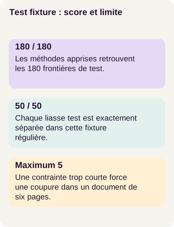
The test contains 50 bundles, 600 pages, and 550 internal decisions. The count is straightforward: each bundle of n pages contributes n - 1 decisions; overall, 600 - 50 = 550. Of these positions, 180 are true boundaries.
Precision asks: how many predicted splits are correct? Recall asks: how many expected splits did we find? F1 is their harmonic mean: 2 × precision × recall / (precision + recall).
To read results directly from counts, we can also write F1 = 2 × TP / (2 × TP + FP + FN). Here, TP counts recovered true boundaries, FP counts over-segmentations, and FN counts merges caused by a missed boundary.
Finally, an exact bundle requires every range to be correct. A single wrong split makes the bundle fail this criterion, even if all other decisions are right. Boundary F1 and the fraction of exact bundles therefore answer different questions.
Results of the r002 workflow
The table reproduces the published counts. Both learned methods have identical quality results on this test, so they share a column without being treated as the same implementation.
| Metric | Page-numbering rule | MLP + threshold 0.5 / MLP + dynamic decoder |
|---|---|---|
| True boundaries recovered | 109/180 | 180/180 |
| Over-segmentations | 22 | 0 |
| Merges | 71 | 0 |
| Boundary F1 | 0.700965 | 1.00 |
| Entirely exact bundles | 30/50 | 50/50 |
| Recovered boundaries between documents of the same type | 53/89 | 89/89 |
Recalculate the simple rule's result. It predicts 109 + 22 = 131 splits. Precision is therefore 109/131, approximately 0.8321, and recall is 109/180, approximately 0.6056. F1 is 218/311, or 0.700965 after rounding. The first two values are calculated from published counts, not a new experiment.
The rule gives 30 entirely exact bundles out of 50, or 60%. It finds only 53 of the 89 boundaries between documents of the same type. A reset to 1 is a pagination clue, not a case identifier: this is the concrete weakness revealed by the comparison.
The MLP with the validation-selected threshold and the dynamic decoder both reach F1 = 1.00, with no over-segmentation or merges. Dynamic programming therefore provides no quality gain on the main test. Here it adds a length policy, not a demonstrated precision benefit.
Computation time and scope of the result
Dynamic decoding takes approximately 0.000060 seconds per bundle, compared with 0.000016 seconds for thresholding. That is roughly 60 and 16 microseconds. These times concern decoding, not PDF reading, MiniLM encoding, training, or the complete export.
The observed workflow took 485.526 seconds, with a public Docker cache, including 35 tests in 8.78 seconds. This is neither a cold-start measurement nor a performance commitment for another machine.
A synthetic dataset prepared for a test is often called a fixture. Here, content, references, and teams follow highly regular patterns. MiniLM remains frozen; only one random seed is used. The presented results include neither OCR—recognizing text from images—nor human review.
The perfect score therefore describes this fixture. It demonstrates neither success on scans, robustness to your users' documents, nor the usefulness of the same length limit in another context.
Summary before the exercise
We have built three separate levels. Text and geometry provide observations. The MLP learns a score at each split position, then thresholding or dynamic programming selects ranges. Finally, evaluation compares splits with annotations and separately checks exported pages.
The key distinction is now this: a solution can be optimal for the algorithm yet wrong for the document. This happens, in particular, when a constraint forbids the correct partition. The exercise will isolate that situation without changing the model.
Exercise: a constraint can forbid the correct answer
Predict before running
Imagine a twelve-page bundle made of two six-page documents. The reference expects ranges [0, 6] and [6, 12]. The model supplies eleven logits favoring this separation.
But the configuration imposes maximum=5. Can the decoder still preserve a six-page document? Is very high confidence enough to override the limit? Write your answer before running the command, then predict what changes if the limit becomes 8.
docker compose run --rm tutorial python -m pdfbundles.cli exercise --config configs/exercise.yaml
Observe, then explain
The correct partition is impossible with a limit of 5: no six-page segment is admissible. This is not necessarily an MLP error. The search is simply not allowed to return the two complete documents.
In the supplied exercise, decode is rerun on the same eleven logits, with limits of 5 then 8. No model is retrained, and the main test is not used.
With 5, the result retains the true boundary but adds two over-segmentations. This gives one correct split among three predicted: precision 1/3, recall 1, then boundary F1 = 0.5. Four segments replace the two expected documents.
Why four segments when three would suffice to cover twelve pages with a limit of five? Because covering all pages is not the only criterion. To retain the true boundary after page six, each six-page document must itself be split at least once. That is what happens in this exercise; simply dividing the total page count by the limit does not describe the selected partition.
With 8, six-page ranges become admissible again and are recovered here: F1 = 1. The limit permits this answer; it does not instruct the decoder to create eight-page documents.
Relaxing a constraint expands the possible solution set but does not guarantee recovery of the reference in every bundle. In this exercise, scores favor the correct solution once it is permitted again. On another document, erroneous scores might favor an incorrect merge.
The lesson is therefore not “choose 8 for every PDF.” Define a policy compatible with the expected documents, then measure it on a separate dataset before using it.
Figures, milestones, and cleanup
Read outputs before erasing them
Consult outputs/evaluation.json for metrics and outputs/exports.json for export checks. Also open the PDFs in outputs/separated/ and the available PNGs. Return to a specific bundle: are the boundaries correct, and was each page exported to the right place?
The following commands generate figures from existing results, check milestones, then clean outputs. Save useful files before running cleanup, because exported PDFs will also be deleted.
docker compose run --rm tutorial python lesson/figures/plot.py
docker compose run --rm tutorial python scripts/check_checkpoints.py
docker compose down
docker compose run --rm tutorial python scripts/clean.py --outputs-only
docker compose down
The milestone check compares copies of educational source files. It does not replace the training-state comparison already performed by verify-resume.
The first docker compose down is intentionally placed before clean in the r002 workflow. clean --outputs-only displays and then removes only outputs/; sources, corpus, and assets remain. The final down ends the workflow. There is no need to globally purge your other Docker projects.
Diagnose at the right level
The GPU works under Linux but not inside the container? Revisit preflight and environment diagnostics. The issue is then GPU access from Docker, not the boundary decision.
Acquisition rejects a file? Check available space and size and fingerprint checks. Substituting another model would change the experiment instead of solving reproducibility.
Resumption differs from the continuous run? Preserve states and check messages before any cleanup. Similar F1 is not enough to conclude that resumption is identical.
Exports are faithful but documents are incorrectly grouped? Inspect scores and the length limit. It is segmentation that needs explaining; page copying may have worked perfectly.
Move from the course to an application
Start with authorized, representative bundles, reliable annotations, and a held-out test set. Define admissible lengths with teams who know the documents. A limit chosen only to simplify computation can forbid a perfectly normal item.
Plan review for low-confidence cases or seemingly incompatible lengths. In a back-office interface, this could take the form of previews of pages on either side of a split, with an option to confirm or move it. This interface is a possible adaptation, not a feature demonstrated by the r002 workflow.
Add dedicated checks when documents contain signatures, forms, annotations, scans requiring OCR, or accessibility requirements. Checking fixture text and pixels does not replace these verifications.
The guiding principle remains simple: the model supplies clues, the decoder applies a policy, and evaluation separately checks segmentation correctness and export fidelity.
Download the r002 course: r002 ZIP.
Further references
The links to Sentence Transformers, PyTorch, NumPy, Python, Docker, and NVIDIA clarify the operations explained throughout the article. The small numerical examples are educational; Atlas results remain those of the r002 workflow. To reproduce it, retain the ZIP's commands, configurations, and pinned files rather than replacing them with installation examples from current documentation.