





Imagine a small 3D tool in a web application. You move a point around a swim ring and want to know: is it inside the material, in the central hole, or outside? How far away is the nearest surface?
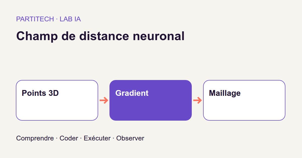
One way to represent the object is to store its vertices and the triangles connecting them: a mesh. We will explore another representation. Instead of asking the network to produce triangles directly, we teach it a function: give it three coordinates, and it returns a signed distance.
The sign indicates which side of the surface the point is on. The absolute value gives its distance from that surface. From this function, we can inspect cross-sections of the object and then extract a mesh.
The tutorial asks a precise question: is learning the right distances enough, or does an additional rule about how they vary through space improve the result? We will compare both approaches on a shape with known geometry. That lets us verify answers rather than simply judging whether the object looks like a swim ring.
Download the tutorial archive.
What we are building
Our target shape is a torus: imagine a circular tube closed on itself, like a swim ring. Its major radius is R=0,55, running from the object's center to the tube's center. Its minor radius is r=0,18, measuring tube thickness from its center to its surface.
Coordinates belong to the experiment, with no imposed physical unit. A distance of 0,01 therefore does not automatically mean a centimeter or millimeter.
We train an MLP, or multilayer perceptron: a network of fully connected layers. Its contract resembles a function in your application: input (x, y, z), numerical output. That output, a scalar, should be negative inside the material, positive outside, and zero on the surface.
Two models start from exactly the same initialization and see the same point batches. The first learns only to recover reference distances. The second receives the same examples but adds an eikonal penalty, weighted by λ=0,1. We will explain this term carefully: it requests not a second shape, but a particular behavior of the function between points.
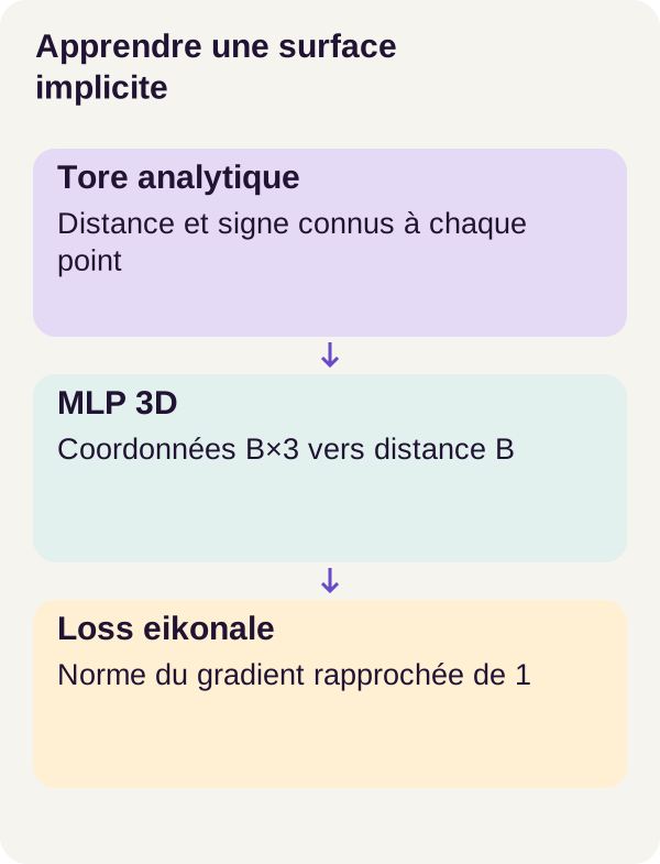
The workflow produces two learned fields, their measurements, and extracted meshes. It also checks that interrupted training resumes correctly. It does not build a web interface, read scans, or reconstruct a real object from photographs.
Why train a network when we already know the torus formula? For this particular object, the formula is an excellent direct solution. Here it serves as a reliable reference: it lets us learn the neural mechanism, detect errors, and understand the penalty's effect. The tutorial does not aim to show that AI advantageously replaces this formula.
Useful concepts
A field: a value for every position
A field associates a value with a position. Think of a function giving temperature at different places in a room. Here, the value is not temperature but signed distance to the torus surface.
An SDF, or signed distance function, uses this convention: −0,05 means “inside the material, 0.05 units from the surface”; +0,05 means “outside the material at the same distance”; 0 denotes the surface itself.
Watch the ring's hole: the object's center is not necessarily inside its material. In our torus, the origin (0, 0, 0) lies in the hole. Its signed distance is positive.
Here are some values calculated directly from the torus formula, not predicted by the network. Coordinates in parentheses use decimal points to avoid confusing numbers with axes.
Point (x, y, z) |
Analytical signed distance | Interpretation |
|---|---|---|
(0.55, 0, 0) |
−0,18 |
Tube center: inside the material. |
(0.73, 0, 0) |
0 |
Outer surface, since 0,55 + 0,18 = 0,73. |
(0.37, 0, 0) |
0 |
Inner surface, facing the hole. |
(0, 0, 0) |
+0,37 |
Hole center: outside the material. |
(0.78, 0, 0) |
+0,05 |
0.05 units beyond the outer surface. |
(0.55, 0, 0.18) |
0 |
Top of the tube. |
These values are geometric calculations. With floating-point numbers, a theoretical zero may appear as a very small value near zero.
A learned function instead of a triangle list
In a fully connected layer, each unit receives every value from the previous layer and combines them with adjustable coefficients. Nonlinear transformations let the network represent more than a simple plane; the exact network is supplied in the project.
Weights are the network's adjustable numbers. During training, they change to bring predicted distances closer to known distances. Once trained, the model uses these weights to answer for new coordinates: this is inference.
We write this function as fθ(x, y, z), where θ represents all learned parameters. It defines an implicit representation: the surface is not stored directly as a list; it is defined by fθ(x, y, z) = 0.
An isosurface groups points to which a function assigns the same value. We are interested in level zero to recover the object's boundary. Similarly, fixing z=0 lets us study a planar cross-section of the field.
DeepSDF presents continuous representation through signed distances. Our experiment is much narrower: one torus and analytical distances, not a reproduction of that paper's entire method.
The network can be queried at coordinates absent from its training set. This does not mean it is exact everywhere: we must measure errors and not assume reliability beyond the studied domain.
The spatial gradient: in which direction does the value change?
Move our point slightly. If the predicted distance changes significantly, the function has a steep slope in that direction. If it changes little, the slope is shallow.
The spatial gradient, written ∇xfθ, collects the three derivatives with respect to coordinates. Here, x denotes the whole point, not just its first axis. The result is a vector of three numbers: variations along x, y, and z.
Its L2 norm is its length: for a gradient [a, b, c], it is √(a² + b² + c²). For example, [1, 0, 0] has norm 1; [2, 0, 0] has norm 2.
For a true signed distance, this norm is 1 wherever the function is differentiable. Intuitively, near a regular surface, moving a short distance perpendicularly changes the signed distance by the same amount. This is not true for arbitrary movement: sliding along the surface does not produce the same change.
Some special positions have no unique nearest-surface direction. This property should therefore not be read as requiring perfect differentiability at every point in space.
The eikonal penalty: a preference, not a guarantee
The penalty encourages the network to have a gradient norm close to 1 at sampled points. This is regularization: we specify not only which answers to learn, but also a desired property of the function.
The tutorial's formula is:
Total loss = distance MAE + λ × mean((‖∇xfθ(x)‖₂ − 1)²).
The loss is the number training seeks to reduce. MAE, or mean absolute error, averages absolute differences from reference distances. The second term penalizes norms too far from 1. With λ=0,1, this value is multiplied by 0.1 before addition; that does not mean it contributes exactly 10% of total loss.
Why retain reference distances? Consider two simple functions: f(x,y,z)=x and g(x,y,z)=x−0,3. Both have a gradient norm of 1, but their zero surfaces lie at x=0 and x=0,3 respectively. The function h(x,y,z)=−x preserves the same plane as f while reversing inside and outside.
The gradient norm alone therefore neither positions the correct surface nor selects its sign. In our experiment, supervised distances provide that information. Implicit Geometric Regularization offers further insight into gradient constraints; its reconstruction protocol differs from our analytical torus.
One programming challenge remains: for this penalty to modify weights, PyTorch must differentiate a computation that already contains a gradient. That is the role of create_graph=True, which we will follow in the code.
Docker and GPU prerequisites
You should be able to read Python functions, work with arrays, and run terminal commands. Neural geometry concepts are introduced here; no prior SDF experience is needed.
The intended workflow uses Linux x86_64, Docker Compose, NVIDIA Container Toolkit, a 24 GiB RTX 3090, 16 GiB of RAM, and 16 GiB of disk space, excluding shared Docker layers. VRAM belongs to the graphics card and is distinct from machine RAM. Keep these conditions to follow the presented workflow, rather than interpreting the explanations as validation of another configuration.
To choose a card, export GPU_DEVICE=0 or its UUID before the sequence. The UUID is its identifier and selects a specific card. The environment check initializes CUDA, NVIDIA's computing environment used here, and runs a computation inside the container.
Seeing a card from Linux is not enough to establish that Docker can use it. The official NVIDIA Container Toolkit guide documents this integration with the host driver.
GPU computations run without networking. Containers apply a read-only filesystem, no-new-privileges, dropped Linux capabilities, and CPU, RAM, and PID limits. These settings bound process permissions and resources; they do not replace model tests.
A checkpoint saves state to recover a model or resume training. Workflow checkpoints are produced locally: do not load them from arbitrary sources. Their trustworthiness also depends on provenance.
Data: verifiable geometric ground truth
Three point sets, three responsibilities
An annotation, or label, here is a signed distance computed with the exact formula. It is neither a human-selected category nor an answer supplied by another model.
The program prepares three sets using distinct seeds. A seed initializes the pseudorandom generator, allowing the same draws to be reproduced within the project's environment.
| Set | Number of points | Role |
|---|---|---|
Training, or train |
65,536 | Supply examples used to adjust weights. |
| Validation | 16,384 | Observe errors on a set separate from training. |
| Test | 32,768 | Measure the results presented later. |
Each set contains half uniformly distributed points in the cube [-1,1]³ and half points constructed near the surface. The former explore the volume; the latter concentrate some learning near the boundary of interest.
A 64³ grid is reserved for extraction. That is 64 × 64 × 64 = 262 144 evaluation positions, not 262,144 additional training examples. It is never used to train the network.
Reading the two functions without confusing them
In the snippet, np means NumPy; R and r are the two radii defined above. The complete project supplies imports and constants.
generate_points() creates coordinates. torus_sdf() then computes reference distances for supplied coordinates. The first function does not itself return labels, and neither function saves files: sequencing and saving belong to the project's preparation stage.
def torus_sdf(points):
    return (
        np.sqrt(
            (np.sqrt(points[..., 0] ** 2 + points[..., 1] ** 2) - R) ** 2
            + points[..., 2] ** 2
        )
        - r
    )


def generate_points(n, seed, std=0.04):
    rng = np.random.default_rng(seed)
    uniform = rng.uniform(-1, 1, (n // 2, 3))
    u = rng.uniform(0, 2 * np.pi, n // 2)
    v = rng.uniform(0, 2 * np.pi, n // 2)
    surface = np.stack(
        [
            (R + r * np.cos(v)) * np.cos(u),
            (R + r * np.cos(v)) * np.sin(u),
            r * np.sin(v),
        ],
        -1,
    )
    near = np.clip(surface + rng.normal(0, std, surface.shape), -1, 1)
    return np.concatenate([uniform, near]).astype("float32")
How does the formula recover a distance?
The expression points[..., 0] selects x coordinates; indices 1 and 2 select y and z. The ellipsis preserves preceding dimensions, allowing computation across an array of points.
Read the calculation in three stages. √(x²+y²) first gives distance from the torus's vertical axis. Subtracting R then centers that distance on the circle through the tube's center. Finally, √((√(x²+y²)−R)²+z²)−r measures the offset from the tube's surface.
Take point (0.78, 0, 0). Its distance from the axis is 0,78. Subtract 0,55 to obtain 0,23, then subtract tube radius 0,18. The result is 0,05, positive. We are indeed outside.
At (0.55, 0, 0), the same calculation gives 0−0,18=−0,18. In the hole, at the origin, it gives 0,55−0,18=0,37. The same formula therefore explains all three situations without a separate rule for the hole.
Why add noise to coordinates?
uniform contains n // 2 points distributed in the cube. Angles u and v then construct the same number of positions on the torus surface: u goes around the ring, and v around its tube. np.stack(..., -1) combines the three coordinates on the final axis.
The program adds Gaussian noise to these positions: random displacements centered on zero. The std=0.04 parameter is their standard deviation per coordinate, not a maximum permitted distance from the surface; the NumPy Generator.normal documentation specifies this convention. np.clip brings coordinates into [-1,1]. Finally, both groups are combined and converted to float32, floating-point numbers stored in 32 bits.
A useful nuance: angles are sampled uniformly, but this is not uniform area sampling across the entire torus surface. The protocol uses this specific generator; we do not attribute another distribution to it.
Noise moves points, not their reference answers. Once coordinates are obtained, their distances are recomputed using the analytical formula. We are therefore not simulating noisy distance annotations such as a sensor might produce.
Preparation saves the datasets and checks that points differ across splits. All three sets still concern the same torus and generation mechanism: a good test result does not measure the ability to learn every 3D shape.
Installing and checking the environment
Extract the archive and place your terminal at its root. Every following command starts from this same directory. Python snippets explain the mechanism; the ZIP supplies the surrounding project.
Start by preparing and checking the environment:
sh scripts/setup.sh
docker compose config --quiet
docker compose build acquire gpu
docker compose run --rm acquire python scripts/acquire.py --config configs/minimum.yaml
docker compose run --rm gpu python scripts/check_environment.py --config configs/minimum.yaml
docker compose run --rm gpu python -m pytest -q
setup.sh prepares the project. docker compose config --quiet checks Compose configuration; build builds images used by the acquire and gpu services.
The name acquire may recall tutorials that download pretrained models. Here, it validates a manifest with no weights to download: we will learn the field from locally generated points. This does not mean Docker image building never needs networking.
The environment check must pass before training. The pytest command then runs the supplied tests. A pass at this stage checks the program and environment; it does not yet prove that the learned network correctly represents the torus.
Now prepare data, inspect the network contract, and check the loss:
docker compose run --rm gpu python -m neural_sdf.cli prepare --config configs/minimum.yaml
docker compose run --rm gpu python -m neural_sdf.cli inspect-model --config configs/minimum.yaml
docker compose run --rm gpu python -m neural_sdf.cli check-loss --config configs/minimum.yaml
The notation B×3 → B means: for a batch of B three-coordinate points, obtain one distance per point. For example, ten points enter as a 10×3 array; ten distances should emerge.
In PyTorch, these arrays are tensors: numbers organized into dimensions that the program can process on the GPU. A scalar loss is a tensor containing just one value.
This shape check is not decorative. With prediction and labels both shaped B, subtraction compares each prediction with its label. Subtracting a B array from a B×1 array may automatically expand to B×B: the program would then compare every pair instead of corresponding pairs only. This is PyTorch broadcasting, not a correct measurement of our distances.
check-loss verifies another contract: the penalty must actually have a gradient toward the weights. Let us see how that check is built.
Core code: making the eikonal penalty trainable
Two gradients, two questions
In web development, the same data may pass through several functions before being saved. Here we must also follow a chain, but a chain of differentiable computations.
The spatial gradient asks “how does distance change if I move the point?” The loss gradient with respect to parameters asks “how does loss change if I change the weights?” The optimizer uses the latter to adjust the network.
The penalty connects them: it depends on the spatial gradient, which itself depends on weights. Learning this property requires preserving that dependency during computation.
The computation graph records operations and dependencies: which result comes from which numbers, multiplications, or other transformations? PyTorch uses it to propagate derivatives. It is not a chart displayed on screen.
def sdf_eikonal_loss(model, points, labels, weight=0.1, create_graph=True):
    points = points.detach().requires_grad_(True)
    prediction = model(points)
    gradient = torch.autograd.grad(prediction.sum(), points, create_graph=create_graph)[
        0
    ]
    distance = (prediction - labels).abs().mean()
    eikonal = (gradient.norm(dim=-1) - 1).square().mean()
    return distance + weight * eikonal, distance, eikonal


def check_loss(config):
    model = torch.nn.Linear(3, 1, bias=False).cuda()
    with torch.no_grad():
        model.weight.copy_(torch.tensor([[2.0, 0, 0]], device="cuda"))
    x = torch.randn(10, 3, device="cuda", requires_grad=True)
    gradient = torch.autograd.grad(model(x).sum(), x, create_graph=True)[0]
    penalty = (gradient.norm(dim=-1) - 1).square().mean()
    weight_gradient = torch.autograd.grad(penalty, model.weight)[0]
    assert torch.allclose(weight_gradient, torch.tensor([[2.0, 0, 0]], device="cuda"))
    return {
        "affine_gradient": [2.0, 0, 0],
        "penalty": float(penalty),
        "weight_gradient": weight_gradient.tolist(),
    }
Following sdf_eikonal_loss()
Prepare coordinates. points.detach() cuts any existing computation history; requires_grad_(True) then requests tracking output variations with respect to those coordinates. This neither freezes model weights nor moves points. It prepares inputs for derivative computation. The detach() documentation specifies this break with the previous graph.
Predict distances. model(points) applies the network to coordinates. Under the B×3 → B contract, prediction and labels carry one value per point.
Compute the spatial slope. torch.autograd.grad() receives the sum of predictions and coordinates. For this network, which processes each point independently of other batch points, differentiating the sum recovers each prediction's gradient with respect to its own point. The result has shape B×3.
The [0] at the end selects the first item in PyTorch's returned tuple, corresponding to points. It does not select only the batch's first point. The torch.autograd.grad documentation describes this computation and its parameters.
Compute both errors. (prediction - labels).abs().mean() gives distance MAE. gradient.norm(dim=-1) computes one norm per point by combining its three derivatives. Subtract 1, square the difference, and average: that is the eikonal penalty.
Return the total and its components. The function returns three tensor-valued numbers: total loss, MAE, and unweighted penalty. Retaining them separately reveals which component improves or deteriorates.
The function does not itself update weights. A later loss.backward() call computes their gradients; the optimizer then updates them. Do not confuse calculating a loss, calculating its gradient, and applying a parameter change.
A loss calculation you can work out by hand
Here are three fictional predictions chosen to explain the formula. They come from neither the trained model nor result files.
| Point | Reference distance | Fictional prediction | Absolute difference |
|---|---|---|---|
(0.55, 0, 0) |
−0,18 |
−0,16 |
0,02 |
(0.73, 0, 0) |
0 |
0,01 |
0,01 |
(0.78, 0, 0) |
0,05 |
0,02 |
0,03 |
MAE is (0,02 + 0,01 + 0,03) / 3 = 0,02.
Now suppose that the norms of the predicted gradients at these three points are respectively 0,8, 1,0, and 1,2. The penalty is ((0,8−1)² + (1−1)² + (1,2−1)²) / 3, or about 0,026667.
With λ=0,1, the total loss is therefore 0,02 + 0,1 × 0,026667 ≈ 0,022667. We do not add 0,026667 directly: the weighting matters.
Why create_graph=True is essential here
PyTorch can calculate a numerical gradient without retaining every dependency needed to differentiate it again. Yet the penalty depends precisely on a gradient that we then want to differentiate with respect to the weights.
create_graph=True builds the graph for the derivative calculation. The path therefore remains available: weights → distances → spatial gradients → penalty. With False, we can still obtain a number for the penalty, but cannot use that path to train the weights.
The official Double Backward with Custom Functions tutorial explores the distinction between calculating a derivative and being able to differentiate its calculation. This supplement explains the mechanism; it does not ask you to replace the project code with a custom autograd function.
Reading the affine test: why do we expect [2, 0, 0]?
check_loss() chooses a linear layer with three inputs, one output, and no bias. It sets its weights to [2, 0, 0]. The computed function is therefore simply f(x,y,z)=2x.
At any point, its spatial gradient is [2, 0, 0]. Its norm is 2 and the penalty is (2−1)²=1. The ten random points do not complicate this check: the slope is constant for this function.
But the test goes further: it differentiates the penalty with respect to the weights. Near the positive coefficient a=2, for a function f(x,y,z)=a×x, the penalty is (a−1)². Its derivative is 2×(a−1), hence 2 at a=2. The other two components are zero. This explains the assertion on [[2.0, 0, 0]].
The spatial gradient and the gradient toward the weights have the same numerical values here, but they are two different objects. The first describes variation in space; the second verifies that regularization can take part in learning.
The check concerns the penalty alone, without multiplication by λ. It therefore expects 2 on the first weight, not 0,2. A plausible numerical loss output would not be enough to replace this assertion.
Train, resume, evaluate, and extract
We can now follow the complete sequence. The first command trains the eikonal variant. The second trains the distance-only variant, which serves as a point of comparison.
The following commands interrupt training after step 500, resume from the saved state, compare the resumed run with the reference run, evaluate both fields, and then extract their isosurfaces.
docker compose run --rm gpu python -m neural_sdf.cli train --config configs/minimum.yaml
docker compose run --rm gpu python -m neural_sdf.cli train --config configs/minimum.yaml --variant distance
docker compose run --rm gpu python -m neural_sdf.cli train --config configs/minimum.yaml --stop-after 500 --run-name interrupted
docker compose run --rm gpu python -m neural_sdf.cli train --config configs/minimum.yaml --resume artifacts/checkpoints/interrupted/state.pt --run-name resumed
docker compose run --rm gpu python -m neural_sdf.cli compare-resume --config configs/minimum.yaml
docker compose run --rm gpu python -m neural_sdf.cli evaluate --config configs/minimum.yaml
docker compose run --rm gpu python -m neural_sdf.cli mesh --config configs/minimum.yaml
A batch is a group of points processed together. An initialization sets the weights before their first update. Starting both variants from the same weights and presenting them with the same batches reduces incidental differences in the comparison: we are studying the added penalty, not two different example sets.
Resuming requires more than the final weights of a layer. The optimizer state and pseudorandom generator state are part of the controlled run. It is comparable to resuming an application process: recovering the latest result is not enough if you have lost the state that determines the next operation.
The results published later come from the validated reader reproduction of this sequence. The tutorial provides neither a reference training duration nor a speed comparison between variants: do not infer a time gain from the quality scores alone.
How do we get from a function to triangles?
The mesh step evaluates the field on its independent 64³ grid, then extracts level zero. The principle of marching cubes is to scan grid cells and build triangles from values that surround the requested level. The scikit-image documentation describes this extraction and the vertices and faces it returns.
A one-dimensional analogy helps explain interpolation. On a segment of length 0,1, suppose endpoint values are −0,02 and +0,03. Linear interpolation places zero at 0,02 / (0,02 + 0,03) = 0,4 of the segment, or 0,04 from the first endpoint. This example explains the principle; it is not a measurement of the tutorial mesh.
The mesh is a discrete approximation of the learned field. Grid resolution affects what can be seen or missed. Increasing that resolution does not retrain the network and does not automatically correct its distances.
Measurements before results
Overall MAE: does the network give the right distances?
Distance MAE averages |prediction − reference| over the evaluated points. A positive error and a negative error do not cancel each other out. The lower this average, the closer the predicted values are to the analytical distances in the population considered.
It is evaluated on validation and on test data. It retains the coordinate unit of the experiment: it is neither a percentage nor a rate of points correctly classified as inside or outside.
MAE near the surface: how does the boundary behave?
The calculation keeps only points whose analytical distance satisfies the proximity threshold declared in the project. Errors are then averaged over this subpopulation.
The numerical threshold is not reproduced in this text: consult the supplied run rather than choosing one after reading the results. Crucially, selection relies on the reference distance, not on the distance estimated by the model itself. An incorrect prediction must not be able to exclude itself from its own evaluation.
Do not confuse “half the generated points are near the surface” with “the number of points retained by this threshold.” Gaussian displacements do not form a strict band; some uniform points may also be near the surface. The published count of 13 832 points comes from evaluation selection, not simply from dividing 32 768 by two.
Gradient-norm error: does the slope have the right length?
This metric averages the absolute difference |‖∇f‖₂−1|. It is not the training penalty, which averages squared differences.
Take again the instructional norms 0,8, 1,0, and 1,2. The mean absolute error is (0,2 + 0 + 0,2) / 3 ≈ 0,133333, whereas the squared penalty is about 0,026667. The two numbers describe the same three norms under different conventions; they are not interchangeable.
This metric does not directly check gradient orientation or surface location. The planar functions in our example all had the correct norm despite shifted surfaces or reversed signs.
Mesh measurements: what is the final extracted object worth?
A vertex is a point in the mesh; a face here is a triangle joining three vertices. Their counts describe the extraction output. More triangles do not automatically mean more accuracy.
The mean analytical deviation of vertices measures their distance from the true torus surface: for each extracted vertex, we calculate the absolute value of the analytical SDF and then average it.
These values must be read alongside field MAE: mesh vertices are not the same population as test points. This average distance from vertices to the surface also does not by itself certify that the entire shape was covered, that all triangles are usable, or that the geometric structure is correct.
Observed results
The following values are from reproduction r1 of the tutorial. The instructional calculations above are not included in these measurements.
Comparing the two fields on the test set
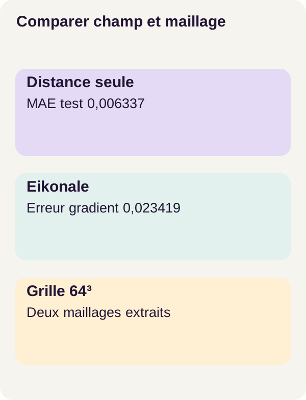
The test set contains 32 768 points. The near-surface measurement covers 13 832 points. For the three metrics below, a lower value is better.
| Test measurement | Distance only | Distance + eikonal penalty |
|---|---|---|
| Overall distance MAE | 0,006337 |
0,008552 |
| MAE near the surface | 0,004770 |
0,004700 |
| Mean absolute gradient-norm error | 0,024407 |
0,023419 |
The eikonal variant slightly improves near-surface MAE and gradient-norm error. However, its overall MAE is higher. The additional constraint therefore does not improve every indicator at the same time.
We can make the gaps more concrete by simply subtracting the published values: overall MAE increases by 0,002215, near-surface MAE decreases by 0,000070, and norm error decreases by 0,000988. These are differences calculated from the displayed rounded values, not new measurement campaigns.
The table gives no dispersion across several independent initializations. It supports describing this observed trade-off, not claiming that such a small difference will systematically recur.
Comparing extracted meshes
The same 64³ resolution was used to extract both meshes.
| Extraction measurement | Distance only | Distance + eikonal penalty |
|---|---|---|
| Vertices | 5 448 | 5 864 |
| Faces | 10 896 | 11 728 |
| Mean analytical vertex deviation | 0,005149 |
0,005189 |
The eikonal variant produces more vertices and faces, but its mean analytical deviation of vertices is slightly higher. A denser mesh is therefore not, in this case, a mesh closer to the surface under this measurement.
The slight improvement in near-surface MAE must not be presented as a demonstrated mesh improvement. The first score concerns selected test points; the second concerns vertices from extraction. They are neither the same population nor the same calculation.
Resuming after interruption recovered the parameters with zero maximum error, as well as the optimizer, generator, and shared initialization. This result validates resumption in the tested run; it is not an additional measure of geometric quality.
What we learned
We learned to represent a shape with a coordinate function, then return to triangles. The network does not receive a vague instruction such as “draw a torus”: it learns point–distance pairs whose answer can be checked.
The eikonal penalty adds a preference about the spatial variation of this function. For it to influence the weights, the calculation must retain the ability to differentiate the spatial gradient. That is exactly what the affine test makes visible.
A useful constraint does not guarantee that every score improves. In this experiment, the regularized variant slightly improves two field indicators, while distance only retains the best overall MAE and the lowest mean deviation of extracted vertices.
Finally, three objects must remain distinct: the analytical shape that serves as reference, the neural field that approximates it, and the mesh sampled from that field. The grid can conceal or introduce artifacts without changing the weights. A result on this torus therefore does not validate reconstruction of a real scan.
Exercise: make a hypothesis before running the command
Before running the command, return to the function used in the check: f(x,y,z)=2x. Predict what happens when create_graph=True becomes False.
Write your answers separately: can the distance still be calculated? Can the spatial gradient still equal [2,0,0]? Can the penalty still display 1? And does PyTorch still have the path needed to differentiate this penalty with respect to the weights?
Then run the negative check provided by the project:
docker compose run --rm gpu python -m neural_sdf.cli exercise --config configs/exercise.yaml
Read the check status and compare it with your prediction. The key point is that a penalty value can remain calculable even when its differentiable dependency on the weights is no longer available. An expected check error is useful information, not a reason to conceal the issue and carry on.
“Gradient unavailable” does not mean “mathematical gradient equal to zero.” In our affine case, we can calculate its value by hand: it is not zero. What is missing is the computation path PyTorch needs.
Keep the reference run. The affine case gives you a prediction to verify: observe the status your command actually returns rather than expecting a particular output sentence. The values calculated by hand explain the mechanism; they do not replace that observation.
Adapt and produce
Change one assumption in a separate experiment
One instructional extension is to vary eikonal weighting in a copy of the project while keeping the data, initialization, and grid comparable. Before measuring, note which indicators you expect to change, then run the adapted sequence again.
This proposal has no pre-announced result. Changing λ creates another experiment; its scores must not silently replace those of r1. The archive remains the reference for the parameters and commands of the presented run.
Why a real scan changes the problem
Here, we know the signed distance of any point thanks to a formula. A set of points from a scan does not automatically provide that same information everywhere in space. Acquisition, units, coordinate systems, noise, holes, and how inside and outside are established become subjects that must be addressed explicitly.
Before a real application, you would also need to specify data rights, acceptance criteria, and the mesh's use: visualization, downstream processing, or another need. Rejection thresholds must depend on that use, not only on a favorable visual impression.
Operation also requires access management for artifacts, backups, error and drift monitoring, and load measurements. The supplied code provides neither a scan pipeline, nor clinical or industrial validation, nor an exposed service.
Troubleshooting and cleanup
If CUDA fails, check the driver, selected card, and Docker integration by following the NVIDIA Container Toolkit guide. Then rerun the environment check before changing the network.
If a gradient error occurs, distinguish an incorrect numerical value from a missing differentiation path. Check requires_grad, create_graph, and that gradients have not been disabled around the calculation concerned. Predicting distances without calculating their derivatives and evaluating a gradient penalty do not require the same execution conditions. Do not remove the affine-check assertion to obtain an apparent success.
If no zero level is present in the grid, examine field values, the queried domain, and the loaded model before concluding that learning failed. An extraction cannot reveal a zero crossing that sampled values cannot recover. Do not automatically replace level zero with another threshold: you would change the surface being sought.
After the exercise, generate figures, check checkpoints, preview cleanup, then stop the services:
docker compose run --rm gpu python lesson/figures/plot.py
docker compose run --rm gpu python scripts/check_checkpoints.py
docker compose run --rm gpu python scripts/clean.py --scope generated --dry-run
docker compose down --remove-orphans
--dry-run means cleanup is a preview: it preserves local files. Examine what is announced before any later deletion. The final command stops the project's Compose resources and orphaned containers; it is not a global Docker purge.
Keep the outputs needed for your comparisons, especially before launching a variant of the experiment.
Primary sources and documentation
The references below explore the concepts in more depth. They do not replace the versions and parameters in the archive for reproducing r1 results.
Park et al. — DeepSDF presents continuous representation through signed distances. Gropp et al. — Implicit Geometric Regularization studies geometric regularization through a gradient property. Their experiments are distinct from the analytical-torus experiment presented here.
The PyTorch — automatic differentiation documentation, the torch.autograd.grad reference, and the Double Backward with Custom Functions tutorial explain derivatives and the graphs needed to propagate them. Pages on detach() and broadcasting complement the code reading.
The NumPy — Generator.normal reference describes the Gaussian-noise draw used to move points.
The scikit-image — marching cubes reference details isosurface extraction from a sampled volume. The NVIDIA Container Toolkit installation guide concerns GPU access from containers.