





Imagine the search bar of a spare-parts store. A customer describes their appliance, its version and the part they need. The engine retrieves the right product family… but places an almost-compatible part ahead of the one that exactly meets the request.
The problem is no longer just finding product pages. We also need to order them correctly.
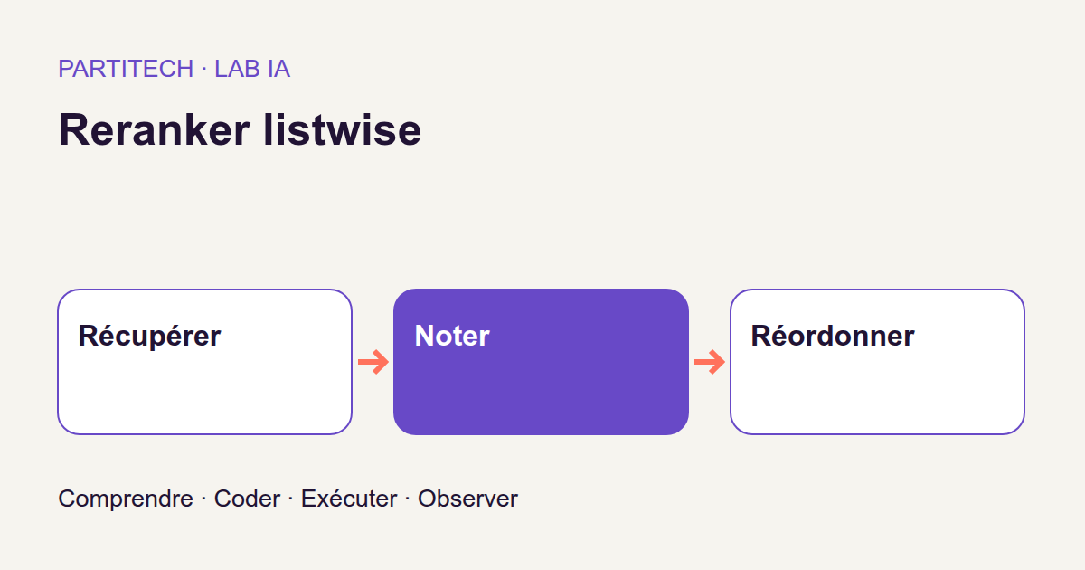
That is the role of a reranker: reread the request alongside each previously retrieved candidate, assign scores, then change their order. For a web developer, the boundary resembles that of a function sorting an array returned by an API: it can move its elements, but cannot retrieve an element the API never sent it.
In this tutorial, we will train this reranking process, understand its computation and measure its limit. Excellent ordering alone cannot repair a list containing no relevant answer.
Download the complete tutorial project
What we are building
We build a synthetic catalog, meaning a fictional catalog created for the experiment. For each request, a lexical search, based on terms in the texts, retrieves eight candidate product pages. A BERT model used as a cross-encoder then assigns a score to each (query, document) pair.
During training, we bring together the eight scores for a query to learn a distribution favoring relevant candidates. This is the listwise approach: the learning function considers the list, not just each pair in isolation.
At the end, candidate identifiers remain the same. Their positions change, not their membership in the list. The program does not write an answer, create a product page or certify the compatibility of a real part.
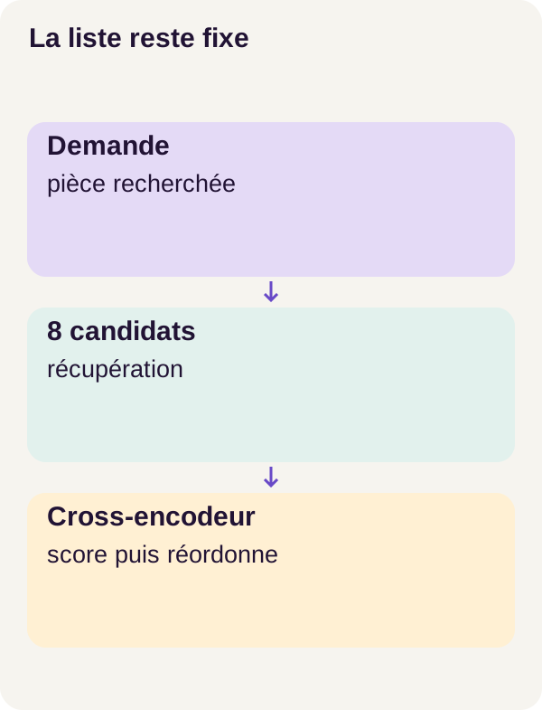
We will compare three rankings: lexical search, a model trained pointwise, and the model trained listwise. We will also check resumption after interruption and read the results in outputs/ranking-metrics.json.
You do not need to know BERT or loss functions to get started. Lists, functions, some Python basics and a terminal are enough to follow the explanations. Running the walkthrough also requires the Docker and GPU prerequisites listed below.
Concepts explained
Retrieval is not reranking
Retrieval answers the question: “Among all product pages, which will we examine?” Reranking then answers: “In what order should we display the selected pages?”
Take an invented example, separate from the r1 corpus. A user is looking for a filter for a fictional Atlas appliance, 2024 version. To simplify the explanation, we show only three candidates, while the actual walkthrough uses eight.
| Illustrative candidate | Reading of the product page | Grade assigned for this example |
|---|---|---|
| A | Fully meets the request | 2 |
| B | Meets only some of the criteria | 1 |
| C | Does not meet the request | 0 |
Search might return the order B, C, A. We would like A, B, C. However, if A is not in the received list, no sorting operation can add it.
Grades are annotations: reference values defined to state what is relevant. The model learns from these values; it does not invent them to grade its own answers. In this tutorial, a “positive” is a candidate with grade 1 or 2. Positive therefore does not necessarily mean fully compatible.
How BERT turns a pair of texts into a score
A model does not compute directly on character strings. The tokenizer splits text into units called tokens, then replaces them with numeric identifiers. A token can be a word, part of a word or a symbol: counting words is not enough to know the length the model will receive.
The pair can be represented schematically as [CLS] query [SEP] product page [SEP]. This is a reading aid, not a tokenization output captured in the experiment. [SEP] separates the two texts; [CLS] is a special position whose representation will be used here to compute the score. The BERT model card describes this input format.
BERT computes numerical representations that account for token context. In our cross-encoder, the query and product page are processed together: their words can therefore interact during this computation. A linear head then transforms the vector associated with [CLS] into a single number. Think of a final function combining the vector's coordinates with learned coefficients.
This number is a score, also called a logit before any transformation into a distribution. It is used to rank pages for the same request. A score of 3 means neither “grade 3,” nor “three times more compatible,” nor “300% probability of compatibility.”
A bi-encoder would work differently: it would encode the query and documents separately, then compare their vectors. A cross-encoder instead reads a pair again for each candidate. That enables direct comparison of the two texts, at an additional computational cost. The Sentence Transformers CrossEncoder documentation presents this reranking architecture.
What “listwise” actually changes
Here, BERT continues to score pairs separately. We do not send it all eight product pages as one long text. It is the loss function that groups their scores by query.
A loss is a number that training seeks to reduce. In a pointwise approach, each pair contributes independently to the objective. In our listwise approach, candidate scores are normalized together: increasing the share assigned to one changes the relative shares of the others.
The objective aligns with our need: we do not just want to recognize several useful pages; we want to give a complete answer more weight than a partial one. This choice remains a hypothesis to evaluate, not a guarantee that listwise will always beat pointwise.
The CrossEncoder loss documentation helps place this family of methods in context. However, the project uses its own graded_listwise_loss function, detailed below. A family name is not enough to know an implementation's exact formula.
From a grade to an expected distribution
The transformation used is gain = 2^grade − 1. For A, B and C, this gives gains of [3, 1, 0]. We then divide each gain by their sum, 4: the target becomes [0.75, 0.25, 0].
In other words, the expected distribution assigns three quarters of its mass to A and one quarter to B. Here, mass simply means a share of a total equal to 1. This is not a business probability: A's grade 2 is known through annotation, not estimated as an event with a 75% chance of occurring.
The target is not a softmax applied to grades. The computation is precisely: grades → gains → division by the sum of gains. Changing this transformation would change the learning objective.
To convert the model's scores into a comparable distribution, however, we use a softmax: p_i = exp(score_i) / sum_j exp(score_j). Values are positive and sum to 1. With three equal scores, each receives one third. With eight equal scores, each receives one eighth.
This normalization is relative to the list. Even eight unsuitable pages can receive eight shares summing to 1. Softmax therefore does not, by itself, detect “no compatible part.”
Training and using the model
Weights are the numerical coefficients learned by the network. During training, scores are compared with targets; backpropagation computes gradients, meaning the sensitivity of the loss to those coefficients. An optimizer uses these gradients to update trainable parameters.
During use, called inference, the model computes scores without receiving the expected grades as information to exploit. Annotations are then used to evaluate the ranking, not to feed it the right answer.
Docker and GPU prerequisites
The r1 walkthrough was defined for Linux x86_64, Docker Compose, NVIDIA Container Toolkit and a 24 GiB RTX 3090. The README specifies 16 GiB of RAM and 16 GiB of disk space. It does not describe a validated CPU walkthrough.
RAM is the machine's memory; graphics-card memory is used for GPU computations. These provisions belong to the project: they do not establish a universal minimum for every card or configuration.
Docker provides the runtime environment. NVIDIA Container Toolkit makes the GPU accessible to that environment; CUDA is the stack used to perform computations on it. A card visible from Linux is not enough: the CUDA check must pass inside the container before training.
The file locks/models.lock.json pins google-bert/bert-base-uncased to revision 86b5e0934494bd15c9632b12f734a8a67f723594. The file locks/environment.lock.json describes the locked environment. For a web developer, these locks play a role comparable to a pinned dependency file: they prevent two installations from silently using different versions.
The acquire service retrieves public assets; the gpu service runs local code. Keep the project's references to reproduce r1: replacing the model or dependencies creates a different experiment.
Data and the central function
Split examples before learning
The synthetic catalog contains 480 documents and 480 queries. The family-based split specifies 336 for training, 72 for validation and 72 for testing. Each list contains eight candidates. Grades 0, 1 and 2 represent incompatibility, partial compatibility and full compatibility, respectively.
Training modifies weights. Validation examines learning choices. Testing provides the final measurement. Splitting by family aims to prevent closely related examples from being used both to learn and to judge the result. Training labels are present only for train candidates.
In a web application, you have probably already used test data with known expected answers. The principle is similar, with an additional constraint: do not train the model on the answers that will be used for its final exam.
The function's inputs and output
A tensor is a numerical array, potentially with several dimensions. Here, scores and grades have one row per query and one column per candidate. For a batch of B queries in the walkthrough, their shape is therefore B × 8.
mask is a boolean array with the same organization. A True value indicates a position to include; False indicates an ignored position. The walkthrough specifies eight candidates per list: the presence of this parameter in the function does not mean its data necessarily contains padding positions.
Here is the continuous excerpt from src/listwise_ranker/losses.py. It assumes PyTorch is imported as torch in its module.
def graded_listwise_loss(scores, grades, mask=None):
    mask = torch.ones_like(grades, dtype=torch.bool) if mask is None else mask
    gains = (torch.pow(2.0, grades) - 1) * mask
    included = gains.sum(-1) > 0
    n = int(included.sum())
    if not n:
        return scores.sum() * 0, {"included": 0, "excluded": scores.shape[0]}
    selected = scores[included].masked_fill(~mask[included], -torch.inf)
    target = gains[included] / gains[included].sum(-1, keepdim=True)
    logp = torch.log_softmax(selected, dim=-1).masked_fill(~mask[included], 0.0)
    return -(target * logp).sum(-1).mean(), {
        "included": n,
        "excluded": scores.shape[0] - n,
    }
This function returns a loss and counters. It does not tokenize any text, call BERT, sort identifiers or update weights itself. It is one step in the training program, not the entire program.
Follow the computation line by line
Create the mask and gains. With no mask supplied, torch.ones_like(..., dtype=torch.bool) includes all positions. torch.pow(2.0, grades) - 1 then transforms grades into gains. Multiplying them by the mask cancels the contribution of ignored positions.
Choose usable lists. gains.sum(-1) adds the gains in each row: -1 means the last dimension, the candidates. included retains rows whose sum is strictly positive. The counter n is therefore a number of included lists, not a number of positive documents.
A list of eight grade-0 candidates has no target distribution to normalize: its gain sum is zero. It is excluded from the loss. That does not mean it should disappear from end-to-end evaluation.
Exclude masked positions. For retained lists, masked_fill replaces ignored scores with -torch.inf, meaning negative infinity. In softmax, their exponential is zero: those positions take no share of the distribution.
Form the target. Each row's gains are divided by their sum. keepdim=True retains a dimension of width 1 so that each row is divided by its own total. Our [3, 1, 0] example indeed gives [0.75, 0.25, 0].
Compute the logarithms of predicted shares. torch.log_softmax directly produces the logarithms of softmax. For numerical stability, this is preferable to computing softmax and then its logarithm separately, as explained in the PyTorch documentation.
The second masked_fill replaces values at ignored positions in logp with 0. Why mask again? Because multiplying 0 × (−inf) does not provide a usable numerical zero: it can produce NaN, a “not a number” value. The ignored position must contribute exactly zero to the final product.
Sum, then average. -(target * logp).sum(-1) computes a loss per list, called cross-entropy here. The final average includes only retained lists. The included and excluded counters let us track that population.
A grade of 0 is not an absent position
We must distinguish two situations. A grade-0 candidate with a True mask remains a competitor in softmax. Its target gain is zero, but assigning it a large share takes that share away from positives and increases the loss. A position masked False is removed from the comparison.
Return to three equal scores and grades [2, 1, 0]. Without masking, the probabilities are [1/3, 1/3, 1/3]. If we mask only the third candidate, the two remaining shares become [0.5, 0.5]. Removing negatives from the denominator is therefore not neutral: it changes the task we ask the model to perform.
There is also an edge case: if the mask removes all positives from a row, that row is excluded from the loss, even if its original grades contained positives.
Calculate the loss by hand
In the A, B, C teaching example, the target is [0.75, 0.25, 0]. For finite scores and active positions, the formula becomes L = −0.75 × ln(p_A) − 0.25 × ln(p_B). ln denotes the natural logarithm. C's zero target gives it no term of its own, but C remains in the softmax denominator.
The distributions below were chosen for explanation; they are not predictions captured during r1.
| Predicted shares A, B, C | Approximate loss | Interpretation |
|---|---|---|
| One third, one third, one third | 1.098612 | All three candidates receive the same share |
| 0.74 ; 0.25 ; 0.01 | 0.572402 | The distribution is close to the target |
| 0.95 ; 0.04 ; 0.01 | 0.843189 | A is favored, but B receives too little weight |
Yet the last two distributions produce the same order: A, B, C. The loss therefore does not only look at who comes first. It compares the entire distribution with the one defined by the grades.
Another consequence: a good loss does not necessarily aim to reach zero. For the target [0.75, 0.25, 0], its lower bound is −0.75 × ln(0.75) − 0.25 × ln(0.25) ≈ 0.562335. With finite scores, C's share remains strictly positive; this bound is approached as that share tends to zero. Seeking zero loss here would mean expecting the wrong result.
A closer look: a positive can receive a gradient that lowers its score
For a single included list, the gradient with respect to each score is predicted share − target share. With three equal scores, it is therefore approximately [-0.416667, +0.083333, +0.333333].
Gradient descent performed directly on these scores would increase A and decrease B and C. Yet B is positive. This is not an annotation error: it currently receives one third of the total, while the target assigns it one quarter. The computation seeks to correct this overrepresentation, not turn B into an incompatible candidate. The actual network then translates these gradients into changes to shared weights; each score is not an independent parameter.
When no list contributes
When n is zero, scores.sum() * 0 returns a zero connected to the score computation, with zero gradient when scores and their sum are finite. The counters indicate that all lists were excluded.
This return value does not mean training has just succeeded or that the optimizer should advance: deciding whether to proceed or skip an update belongs to the calling loop. The excerpt contains no optimizer.step().
Finally, this function is not a general input validator. It does not explicitly check all shapes, score finiteness or whether grades belong to {0, 1, 2}. Keep the project's surrounding contracts and checks, rather than assuming it accepts arbitrary arrays.
Install and prepare the lists
Check the environment before touching weights
Download the ZIP, extract it and open the terminal at its root. All the following commands run from that same directory. They follow the r1 walkthrough in README.md and lesson/tutorial.json.
sh scripts/setup.sh
docker compose config --quiet
docker compose build acquire gpu
docker compose run --rm acquire python scripts/acquire.py --config configs/minimum.yaml
docker compose run --rm gpu python scripts/check_environment.py --config configs/minimum.yaml
docker compose run --rm gpu python -m pytest -q
setup.sh prepares the project. docker compose config --quiet checks the Compose configuration, then build builds the images for the acquire and gpu services. Acquisition retrieves public assets according to the locks. The check_environment.py script then checks CUDA access inside the container.
The final command runs the project's test suite. These tests check the program's mechanics; passing them does not yet mean a product page will be relevant to a real customer's request. At this stage, the goal is a compliant environment and passing checks before learning begins.
The repeated form docker compose run --rm gpu … runs a command in the gpu service, then removes the temporary container when it finishes. It does not mean you should manually enter the container to type the rest.
Prepare, inspect and check the formula
We can now build the lists, examine what the model receives and check the loss on known numbers.
docker compose run --rm gpu python -m listwise_ranker.cli prepare --config configs/minimum.yaml
docker compose run --rm gpu python -m listwise_ranker.cli inspect-pairs --config configs/minimum.yaml
docker compose run --rm gpu python -m listwise_ranker.cli check-loss --config configs/minimum.yaml
After prepare, examine the splits and each list's eight candidates. You must be able to connect a query, its candidate identifiers and the grades used by the protocol. This association must remain stable: if a column changes document without its grade following it, the program would learn to favor the wrong candidate.
inspect-pairs makes truncation to the model's configured length visible. Truncation means removing some tokens when a pair is too long. The limit applies to the pair's input, not just the number of words on the product page. The value used in r1 must be read from the ZIP's configuration.
In our fictional example, a final sentence such as “only for the 2023 version” can be decisive. If it is removed before BERT, it does not contribute to the score. The model may then score an input deprived of essential information, even though the original page contains it.
check-loss checks the computation on known tensors. Connect its result to the grade transformation and gain normalization before starting training. Checking the formula and checking tokenization are complementary: a correct formula does not restore truncated text.
Train, resume and measure
Compare two learning objectives
The first command trains the listwise variant. The second launches the pointwise variant. The next three create an interrupted run, resume it and compare the resumed run.
docker compose run --rm gpu python -m listwise_ranker.cli train --config configs/minimum.yaml
docker compose run --rm gpu python -m listwise_ranker.cli train --config configs/minimum.yaml --variant pointwise
docker compose run --rm gpu python -m listwise_ranker.cli train --config configs/minimum.yaml --stop-after 20 --run-name interrupted
docker compose run --rm gpu python -m listwise_ranker.cli train --config configs/minimum.yaml --resume artifacts/checkpoints/interrupted/state.pt --run-name resumed
docker compose run --rm gpu python -m listwise_ranker.cli compare-resume --config configs/minimum.yaml
Keep this order: resumed depends on the file artifacts/checkpoints/interrupted/state.pt created by interrupted. The --stop-after 20 option sets the interruption point for this test; by itself, it does not give the recipe's total number of updates.
A checkpoint is a saved point in training. Full resumption is more than loading weights to make a prediction: it must recover the state needed to continue computation. The walkthrough provides this check through compare-resume. Consult its output for the result of your run; the ranking measurements below do not replace this resumption check.
The pointwise variant serves as a comparison. Its loss code is not reproduced in this article: do not infer a precise formula from the word “pointwise” alone. To study this implementation difference, use the archive's code while retaining the reference configuration.
Measure the batch, then explain one case
Once training and resumption have been checked, evaluate the rankings before dwelling on a particularly convincing search.
docker compose run --rm gpu python -m listwise_ranker.cli evaluate --config configs/minimum.yaml
docker compose run --rm gpu python -m listwise_ranker.cli inspect-case --config configs/minimum.yaml
outputs/ranking-metrics.json contains aggregates, meaning measurements summarizing several queries. inspect-case then helps review an individual case.
For that case, connect the request, product pages, their grades and their positions before and after reranking. Check that the identifiers remained the same. The case explains part of the result; it is not enough to draw conclusions about the average across 72 test queries.
Metrics before measurements
Coverage@8: is there at least one relevant candidate?
Coverage@8 is the proportion of queries whose eight candidates contain at least one positive:
coverage@8 = number of lists with at least one positive grade / total number of queries.
This measure answers only a presence question. A list whose only positive ranks eighth is covered. So is a list containing only a grade-1 partial match. Coverage therefore means neither “the right part at the top,” nor “all relevant parts retrieved,” nor “full compatibility.”
In a teaching example with four requests, three of which have at least one positive, coverage is 3 / 4 = 0.75. Reordering those same lists does not change this number.
NDCG@5: how good are the top positions?
NDCG, short for normalized discounted cumulative gain, measures accumulated relevance gain, discounted by position, then normalized. Behind the name are three simple ideas: a more relevant page earns more; a lower-ranked page earns less; and the result is compared with an ideal ranking.
The @5 suffix means only the first five positions contribute to the observed score. With nonnegative grades and an ideal defined over the same reference set, 1 corresponds to the ideal and 0 to no gain in the top five positions.
Let's calculate this for our teaching example. We choose gains of 2^grade − 1 and a rank discount of 1 / log2(rank + 1), a convention documented in TensorFlow Ranking. This reference explains the metric; it adds no TensorFlow dependency to the project.
With this convention, DCG@5 = sum of gains at the top five ranks, each divided by log2(rank + 1). log2 is the base-2 logarithm: at rank 1, the denominator is 1; at rank 3, it is 2. Grade 2 therefore earns 3 in first position but only 1.5 in third position.
For the eight grades [2, 1, 0, 0, 0, 0, 0, 0], the ideal order gives:
IDCG@5 = 3 / log2(2) + 1 / log2(3) ≈ 3.630930.
NDCG is then DCG / IDCG. Here are several permutations of the same grades, calculated solely for explanation:
| Grades in the proposed order | Coverage@8 for this query | Illustrative NDCG@5 |
|---|---|---|
| 2, 1, 0, 0, 0, 0, 0, 0 | 1 | 1.000000 |
| 1, 2, 0, 0, 0, 0, 0, 0 | 1 | 0.796708 |
| 0, 1, 2, 0, 0, 0, 0, 0 | 1 | 0.586883 |
| 0, 0, 0, 0, 0, 2, 1, 0 | 1 | 0.000000 |
The last row matters: relevant candidates are present, but too low to contribute to the top 5. The reranker therefore has an opportunity to improve, unlike when none of its candidates is positive.
The project's complete metric computation is not included in the earlier Python excerpt: that computes the training loss. When adapting evaluation, also check which documents define the ideal. Ideally sorting available candidates and comparing against all relevant catalog documents do not always produce the same denominator. The small calculations above explicitly use the eight displayed grades as their reference set.
Finally, two identical orders can have the same NDCG and different losses. That was the case for distributions [0.74, 0.25, 0.01] and [0.95, 0.04, 0.01]: both rank A, B, C, but do not distribute scores in the same way. The loss supports learning; the metric judges the result against a given criterion.
Conditional and end-to-end: two averages, two denominators
Conditional NDCG@5 is computed only over covered lists, where the reranker has at least one positive. It describes ranking in situations where a relevant document was available.
End-to-end NDCG@5 also retains lists without positives in the denominator. In the presented protocol, they contribute zero. This choice makes visible the share of requests for which the system presents no relevant answer.
Return to our four fictional requests. If each of the three covered lists reaches an NDCG of 1, their conditional average is 1. But across all four requests, the average is (1 + 1 + 1 + 0) / 4 = 0.75.
With an unweighted average and this zero convention for uncovered lists, we have:
end-to-end NDCG = coverage × conditional NDCG.
Since conditional NDCG does not exceed 1, coverage sets a ceiling on the end-to-end score. This ceiling is a bound; it is not automatically attainable by any model or with any choice of ideal ranking.
An unanswered query deserves an explicit status
We must still distinguish two possible reasons for a list having no positive: the right page exists in the catalog but was not retrieved, or no catalog page answers the request.
In the first case, improving retrieval may help. In the second, the system must also know how to signal that no answer exists. The chosen protocol retains these cases in the end-to-end score; this is not a universal convention that can diagnose their cause on its own.
Actual results
The r1 measurements
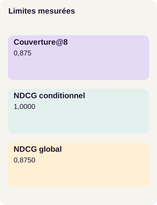
The test covers 72 queries, including 63 covered lists. The report describes the other 9 cases as having “no global positive.” Coverage@8 is 63 / 72 = 0.875.
That wording matters: we must not turn those nine cases into nine correct parts necessarily present in the catalog but missed by search. The number of uncovered lists is not enough to establish that diagnosis.
Here are the published measurements, retained at their original precision:
| Ranking | Conditional NDCG@5 | End-to-end NDCG@5 |
|---|---|---|
| Lexical | 0.9903969127585871 | 0.8665972986637638 |
| Pointwise | 0.8838329034231467 | 0.7733537904952533 |
| Listwise | 1.0 | 0.875 |
Coverage@8 remains 0.875: the rerankers work on the same candidates. Here, the listwise model achieves a perfect conditional order under the metric used. The end-to-end average nevertheless remains limited: (63 × 1 + 9 × 0) / 72 = 0.875.
The values for the other methods follow the same relationship, subject to numerical rounding. For pointwise, 0.8838329034231467 × 0.875 ≈ 0.7733537904952533. There is no contradiction between two different scores: they divide by different populations.
The useful result is not “AI beats search”
Lexical search is already very strong on this corpus: its conditional NDCG is approximately 0.9904. The listwise model improves this result, but the available margin was small. Subtracting the published measurements gives a gain of approximately 0.009603 in conditional NDCG and 0.008403 in the end-to-end score. These are calculated score differences, not new measurements or percentages of compatible parts.
The pointwise variant, meanwhile, ranks worse than the lexical reference in this experiment. Adding and training a model is therefore not an improvement by definition. We must retain a simple reference to check what the new step actually contributes.
Nor does the table establish that listwise will always outperform pointwise. It describes this synthetic corpus, this model and this recipe. It provides neither a latency measurement under load nor evidence of generalization to other catalogs.
What the perfect score does not guarantee
A conditional NDCG of 1 means the top positions satisfy the evaluation's chosen ideal for covered lists. It is not certification of physical compatibility, an absence of unanswered cases or proof that the annotations are perfect.
The main lesson is therefore twofold: learning the order can help, but the order remains limited by the candidates and the definition of relevance. Retrieval, learning and evaluation each have a role; a good number at one stage does not replace the others.
Exercise: predict, then run
Remove the best candidate
Imagine removing A, the best document in our example, while retaining the other candidates' identifiers. Without running the program, make your prediction: can additional training or a very high score make A reappear in this list's ranking?
The supplied scenario performs this comparison without asking you to modify the reference engine.
docker compose run --rm gpu python -m listwise_ranker.cli exercise --config configs/exercise.yaml
The output confirms that the reranker receives and returns the same candidates: it can reorder them, but never retrieves an absent identifier. To check this property, compare identifiers in the list after removal with those in the final ranking. Do not compare them with the original list while forgetting the deliberate deletion.
Be careful with a second prediction: removing the best document does not necessarily make the list entirely irrelevant. If B, with grade 1, remains, the list is still covered. If we removed its only positive, it is no longer covered. In both cases, the absent best document remains impossible to retrieve through reranking alone.
This distinction explains why the exercise first checks a property of identifiers. Better ordering of the remaining candidates would not prove that retrieval had been repaired.
Preserve artifacts before finishing
An artifact is a file produced by the walkthrough: a figure, measurement or training checkpoint. Finish by generating figures, checking checkpoints, previewing cleanup and stopping services, in that order.
docker compose run --rm gpu python lesson/figures/plot.py
docker compose run --rm gpu python scripts/check_checkpoints.py
docker compose run --rm gpu python scripts/clean.py --scope generated --dry-run
docker compose down --remove-orphans
Checkpoints are checked after the exercise. --dry-run requests a preview: clean.py shows what it would target without deleting files. The docker compose down --remove-orphans command stops the project's services; walkthrough files retained on the host remain available.
Adaptation, limitations, troubleshooting and cleanup
From a fictional catalog to your product pages
The first step is not changing BERT. It is writing a definition of relevance reviewed by people who know the catalog. What exactly does “partially compatible” mean? Is it a result to display with a caveat, a useful alternative or a part to exclude from any purchase suggestion? The grading chosen for a tutorial does not replace this business decision.
Version product pages, queries, annotations and splits. Text can change while identifiers remain stable; without a catalog version, you risk comparing an old score with a new page. Also preserve candidate lists to distinguish a ranking change from a retrieval change.
Measure coverage, ranks, truncation and reranking cost separately. Increasing the candidate count changes both what becomes accessible to the model and the number of pairs to process. The new result must be evaluated as a new experiment, not added to r1 figures as if it described the same protocol.
Check languages and what is actually read
The BERT base uncased model card specifies English pretraining and processing that does not distinguish uppercase from lowercase. The name “BERT” therefore does not guarantee automatic adaptation to French requests, technical references or every convention in your catalog. The French example used in the original explanations is not a measured multilingual result.
The cross-encoder's max_length can also remove the decisive part of a page. Text visible in a source file is not necessarily fully visible to the network after tokenization. Inspect pairs before attributing an error solely to learning.
Do not confuse ranking with a decision
The mechanism returns an order, not authorization to purchase or install. Check high-stakes cases before any automation. A real system must in particular handle unanswered requests, uncertain annotations and rules that prohibit certain substitutions.
The listwise target asks for a relative distribution among candidates; here it does not learn a universal compatibility threshold. Designing rejection or human validation requires specific data and checks, separate from improving NDCG alone.
Troubleshoot without silently changing the experiment
The GPU is not visible. Rerun the environment check before training, then check Docker integration using the NVIDIA Container Toolkit guide. Do not silently replace GPU execution with an unvalidated CPU walkthrough.
Acquisition fails. Check the acquire service's network access, fix the cause of failure and rerun the same command. Changing the model revision to work around a missing asset would lose the experiment's reference.
The loss seems unusually low. Reread included and excluded before drawing conclusions. A fully excluded batch returns zero without providing supervision. A mask removing troublesome candidates can also make the objective artificially easier.
Conditional NDCG is excellent, but the overall score plateaus. Look at coverage and requests with no positive. Do not ask the reranker to return pages it never received or create a part absent from the catalog.
You want to clean up experiments. The end-of-walkthrough commands are already given in the exercise. clean.py --dry-run deletes no results; docker compose down --remove-orphans does not replace cleanup of your local files. Inspect and preserve useful measurements before any separate deletion.
We now have a walkthrough connecting an interface need—presenting results better—to a verifiable learning formula. Its conclusion remains concrete: a good reranker puts the right candidates in the right positions; it never removes the need to check which candidates were available.
Official sources
The following references deepen the concepts. To reproduce r1 measurements, keep the archive's versions and configuration: external documentation does not replace them.
- Sentence Transformers: training a CrossEncoder, for pair scoring and training a reranker.
- Sentence Transformers: CrossEncoder losses, for comparing loss families without confusing their implementations.
- BERT base uncased, for the model, its pretraining language and pair representation.
- PyTorch:
log_softmax, for stable computation of log probabilities. This versioned page documents the operation; it does not state the version installed by the project. - TensorFlow Ranking: NDCG definition, for gain normalization and the teaching calculation's conventions, without using TensorFlow in the walkthrough.
- Docker Compose: GPU support and NVIDIA Container Toolkit: installation, for accessing the card from a container.