





You are building a document management screen. Your goal seems simple: suggest a category for each document to make filing easier. You start with a few conditions: a title contains ‘draft’, a paragraph asks for a review, another sentence announces approval.
Then the fictional document V-033 arrives. Its title contains ‘approved’, but its body says ‘for review’. Which rule should you trust? Always giving the title priority does not solve the problem: a title can also contain a negation or an outdated statement.
This is the starting point for weak supervision: using imperfect clues to build training data without treating them as certain answers. Here, we will write rules, learn to combine their opinions, then train a text classifier from the result.
The program suggests classes for fictional documents. It does not change any administrative status or infer real approval from a title. Our question is more modest, but measurable: does this pipeline learn anything useful, or does it perform worse than a simpler method?
Download the complete tutorial project
What you will build
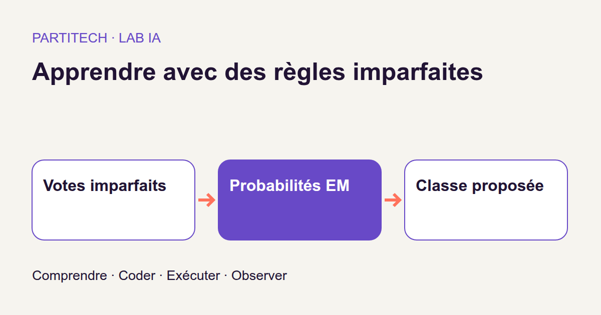
The workflow follows document → rule votes → class probabilities → text classifier → suggestion.
A class is simply a category to predict. A rule can suggest one, or abstain. The first model receives these votes and estimates a probability distribution across the three classes. For example, it may assign more probability to EN_REVUE while still retaining some uncertainty about ANNONCE_APPROUVE.
A second model, the text classifier, then learns from the document text and these distributions. The two models therefore have different inputs: the first combines the rules’ opinions; the second learns to classify text. This tutorial does not use a large language model tasked with writing an answer.
Why not stop at the rules? Because we want to test whether combining them can provide a useful training signal for the classifier. This is a possibility to evaluate, not an established benefit. The general principle is presented in this introduction to weak supervision by the Stanford research team. The ZIP project demonstrates a limited mechanism whose calculations we can follow.
We will compare four methods: majority voting, the model that combines votes, a classifier trained on a few reliable annotations, and the classifier using weak supervision. Along the way, we will explain abstention, latent variables and the EM algorithm without assuming you already know them.
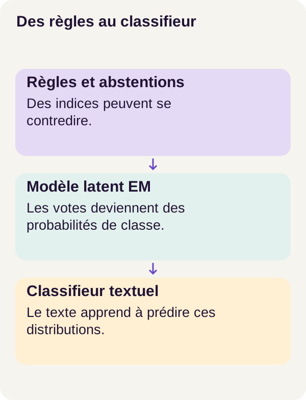
A rule is an imperfect clue, not a reliable annotation.
Prepare a reproducible CPU environment
You need to be able to read Python, use a terminal and run Docker. Here, a numerical array is a set of numbers arranged in rows and columns; we will explain what its dimensions represent at each stage.
This project is validated on CPU, meaning the machine’s processor. No NVIDIA GPU is required. The README recommends 12 GiB of RAM and 6 GiB of working disk space, plus Docker storage. These are preparation guidelines, not guaranteed resource usage measurements.
Extract the ZIP and open a terminal in its root folder, the one containing README.md. All the following commands are run from this directory. Check the environment, prepare the folders, then build the services.
sh scripts/preflight.sh
sh scripts/setup.sh
docker compose config --quiet
docker compose build acquisition tutorial learning inference
The first script performs preflight checks. The second prepares the directories. docker compose config --quiet checks the Compose configuration; build builds the environments required for the workflow. Fix any blocking error before moving on.
The services separate responsibilities: tutorial prepares the data and evaluations; learning receives the training inputs and permitted annotations; inference produces predictions without consulting the expected answers. assets/ stores the learned states and outputs/ the results. The Compose file in the ZIP details the mounts and restrictions.
The model is initialized locally: we will not download pretrained model weights. Here, the acquisition stage checks an empty registry and downloads no third-party weights. It remains part of the workflow, before checking the containerized environment and running tests.
docker compose run --rm acquisition python scripts/acquire.py --config configs/minimum.yaml
docker compose run --rm tutorial python scripts/check_environment.py
docker compose run --rm tutorial python -m pytest -q
The reference workflow reports 24 passing tests. They check program behavior and the rejection of invalid cases. Do not confuse them with a measure of document classification quality: passing tests do not mean every suggested class is correct.
Read the data and annotations
The project’s three classes are BROUILLON, EN_REVUE and ANNONCE_APPROUVE. The last denotes an announcement in a fictional document, not legal approval. Texts may contain negations, outdated statements or misleading titles.
The code represents classes as integers. Here is the small dictionary to keep in mind:
| Value | Meaning |
|---|---|
0 |
BROUILLON |
1 |
EN_REVUE |
2 |
ANNONCE_APPROUVE |
-1 |
Abstention: no class suggested. |
-1 is not a fourth document category. It tells us about a rule or method’s behavior: it abstains.
An annotation, also called a label, specifies an example’s reference class. The corpus contains separate training, validation and test sets. Training adjusts the parameters; validation lets us examine behavior during development; testing measures the final result on separate documents.
The test set contains 360 documents, with 120 reference examples of each class. We also have 90 anchors: training examples with known classes. The word ‘anchor’ describes their role: they provide reliable reference points for the intermediate model. They are also used to train a small comparison classifier without weak supervision.
This is therefore not learning without any annotations. The question is what the rules contribute in addition to these reliable examples.
Let us create the data.
docker compose run --rm tutorial python -m ged_supervision_faible_statuts.cli prepare --config configs/minimum.yaml
Notice the separation between text and annotations. The program can read a document’s title, body and permitted metadata. It must not read its test answer to produce a prediction. The 90 anchors are an explicitly permitted part of supervision; test references remain reserved for evaluation.
Build rules that can abstain
A rule offers an opinion, not certainty
A labeling function is a Python function that looks for a clue and returns a class, or -1 when it has no opinion. For a web developer, think of the distinction between a missing value and a value of zero: here, ‘I don’t know’ must never become BROUILLON by default.
The project has eight rules. Some inspect the title, others the body; another uses an export date. The last deliberately encodes a fragile fictional correlation: a late export does not prove approval.
Here is the central function. Read the article’s excerpts alongside the constants and helper functions in the ZIP; the commands run the complete project.
def apply_label_functions(document):
    title = normalize(document["title"])
    body = normalize(document["text"])
    date = document.get("export_date")
    # Deliberately imperfect: title rule ignores negation, body approval excludes quoted and negated mentions.
    tests = [
        ("valide" in title, 2, "validé dans le titre"),
        ("provisoire" in title or "brouillon" in title, 0, "titre provisoire"),
        ("relecture" in title, 1, "titre relecture"),
        (
            "pour relecture" in body and "pas pour relecture" not in body,
            1,
            "corps pour relecture",
        ),
        ("version de travail" in body, 0, "corps version de travail"),
        (
            "annonce une approbation obtenue" in body
            and "aucune signature" not in body,
            2,
            "annonce positive et absence de négation détectée",
        ),
        (
            bool(date and date >= "2026-08-26"),
            2,
            "export tardif : corrélation fictive, pas approbation",
        ),
        ("commentaires attendus" in body, 1, "commentaires attendus"),
    ]
    return [
        {
            "rule": name,
            "vote": k if active else ABSTAIN,
            "reason": reason if active else "aucun motif reconnu",
        }
        for name, (active, k, reason) in zip(RULES, tests)
    ]
normalize() standardizes case and accents before searching. This makes string comparison easier, but does not give the rule an understanding of the sentence.
Each element of tests contains three pieces of information: a condition, the suggested class number when it is true, and a textual explanation. zip(RULES, tests) associates these elements with rule names. The result retains rule, vote and reason, making it possible to trace an opinion’s origin.
Look at the first condition: it simply searches for valide in the normalized title. It deliberately ignores negation. As an educational counterexample, the French title ‘Non validé’ (‘Not approved’) also contains this string after normalization. The rule can therefore vote incorrectly while executing exactly the intended code.
The body conditions are slightly more selective: one excludes the wording pas pour relecture, another checks for the absence of aucune signature. These are specific string checks, not a general parser for negations or quotations. The excerpt’s comment should be understood within this limited scope.
Finally, 2026-08-26 is the threshold set in the fictional corpus’s export rule. It is neither a date to replace with today’s date nor a business rule to reuse unchanged.
For V-033, the title and body therefore give us conflicting clues. We will retain them rather than hide the conflict behind an arbitrary ordering of conditions.
Start with a simple majority
Before learning to combine rules, let us calculate a reference without training, or baseline: count the votes.
docker compose run --rm learning python -m ged_supervision_faible_statuts.cli baseline --config configs/minimum.yaml
outputs/rules.json describes conflicts and abstentions. Majority voting returns no opinion if no rule votes or if several classes tie for first place. It does not select the first class just to produce an answer.
The votes array has one row per document and one column per rule, making eight columns in the main workflow. The following function converts this array into vote proportions and decisions.
def majority_vote(votes):
    counts = np.stack([(votes == k).sum(1) for k in range(3)], axis=1)
    total = counts.sum(1)
    probabilities = np.divide(
        counts,
        total[:, None],
        out=np.full(counts.shape, 1 / 3, dtype=np.float64),
        where=total[:, None] > 0,
    )
    tied = (counts == counts.max(1, keepdims=True)).sum(1) > 1
    predicted = np.where((total == 0) | tied, -1, counts.argmax(1))
    return probabilities, predicted
For each class k, (votes == k).sum(1) counts the corresponding opinions for each document. np.stack(..., axis=1) gathers these counts into three columns, in the order BROUILLON, EN_REVUE, ANNONCE_APPROUVE. total counts only expressed votes: the -1 values are not added to any class.
total[:, None] gives the total a column shape so that the three counts in a row can be divided by the same number. The where parameter avoids division by zero. When no rule speaks, out supplies a uniform distribution: one third for each class.
But a distribution is not yet a decision. tied detects ties, and np.where imposes a prediction of -1 when the total is zero or several classes win.
Let us take three small teaching examples, limited to three rules to make the calculations easy to read. These are not V-033’s complete outputs.
With votes [1, 1, 2], the counts are [0, 2, 1]. The distribution is [0 ; 2/3 ; 1/3] and the decision is 1, meaning EN_REVUE.
With [2, 1, -1], the counts are [0, 1, 1]. The distribution is [0 ; 0.5 ; 0.5], but the decision remains -1: there is a tie.
With [-1, -1, -1], the distribution is [1/3 ; 1/3 ; 1/3] and the decision is also -1. This time, nobody voted.
The last two cases lead to the same abstention, but for different reasons. Retaining the votes and probabilities makes this difference understandable.
Estimate a hidden class with EM
The problem: knowing the classes to evaluate the rules… and vice versa
Majority voting gives every opinion the same weight. We would like to go further: does a rule often get a class wrong? Does it confuse a draft with a document under review? Does its opinion contribute anything when other rules contradict it?
The difficulty is circular. To know the rules’ errors, we would need to know the documents’ classes. To estimate those classes, we want to use the rules.
A latent variable is information that is not directly observed. Here, it is a document’s reference class when the document is not one of the anchors. The model maintains probabilistic hypotheses about this class rather than immediately deciding it is 0, 1 or 2.
Three arrays to understand
pi contains the estimated class proportions. For example, [0.2 ; 0.5 ; 0.3] means that, without new evidence, the model distributes its probabilities as 20%, 50% and 30%. These values belong to the numerical example provided below; they are not the corpus’s learned proportions announced in advance.
theta describes each rule’s behavior. Its dimensions follow the order rule, latent class, observed vote. With eight rules and three classes, its shape is (8, 3, 3). A cell theta[j, k, c] represents the probability assigned to vote c from rule j when the assumed class is k. An off-diagonal cell therefore represents a possible confusion, not necessarily a programming error.
q contains one distribution per document. With N documents, its shape is (N, 3). A row indicates how plausible each class is under the current parameters. In EM terminology, these values are also called responsibilities: they allow a document to contribute partially to several classes during the update.
Here, theta has no column for -1. Abstentions are ignored in the vote calculation; their frequency is not modeled as a fourth output.
Alternate estimation and updating
EM stands for Expectation-Maximization. The algorithm alternates two operations: the E step estimates q using the current parameters; the M step recalculates pi and theta using these distributions. Anchors retain their known classes throughout this process.
In other words: ‘Given what I know about the rules, which classes are plausible? Then, given those plausible classes, how should I reestimate the rules’ behavior?’
The model makes an important simplification: it assumes votes are independent when the true class is known. This allows their contributions to be multiplied. But two copied rules are not two independent observations: they follow exactly the same clue. We will test this limitation in the exercise.
Add up evidence without losing small probabilities
The calculation starts in logarithms. A logarithm turns a product into a sum: instead of multiplying several probabilities, the program adds their logarithms.
def log_joint(votes, pi, theta):
    result = np.broadcast_to(np.log(pi), (len(votes), 3)).copy()
    for j in range(votes.shape[1]):
        rows = np.flatnonzero(votes[:, j] >= 0)
        for k in range(3):
            result[rows, k] += np.log(theta[j, k, votes[rows, j]])
    return result
np.broadcast_to(...).copy() prepares a row of three scores per document, initialized with log(pi). The loop then iterates over the rules. np.flatnonzero(votes[:, j] >= 0) selects only documents for which rule j expressed an opinion.
For each possible class k, the program adds the contribution of the vote actually observed. It no longer merely counts ‘how many rules chose this class?’; it asks ‘are these votes plausible if this is the correct class?’
At this stage, the scores do not yet form a normalized distribution. That is the E step’s role.
def e_step(votes, pi, theta, anchors):
    validate_inputs(votes, pi, theta, anchors)
    joint = log_joint(votes, pi, theta)
    q = np.exp(joint - logsumexp(joint)[:, None])
    for i, k in anchors.items():
        q[i] = np.eye(3)[k]
    return q
The line that builds q converts a document’s three scores back into probabilities summing to one. logsumexp performs this normalization stably, even with very small probabilities.
Normalization must be performed document by document. Here, logsumexp(joint)[:, None] expects one normalizer per row, to subtract from the three corresponding scores. Keep the project’s helper function: a library function with the same name may require an explicit axis. The SciPy documentation for logsumexp explains this calculation and the axis’s role; it is not an instruction to replace the code.
Finally, np.eye(3)[k] builds a certain target for an anchor. If its known class is 1, its row becomes [0, 1, 0]. The rules cannot substitute their own hypothesis.
For a document with no vote and no anchor, no new evidence has been added: q remains equal to pi. If it is an anchor, its known class takes precedence, even without votes.
Count partial contributions with the M step
Now let us move from these hypotheses to the new parameters.
def m_step_map(votes, q, alpha=1.1):
    if (
        alpha <= 1
        or q.shape != (len(votes), 3)
        or (q < 0).any()
        or not np.isfinite(q).all()
        or not np.allclose(q.sum(1), 1)
    ):
        raise ValueError("Invalid responsibilities or Dirichlet prior")
    pi = q.sum(0) + alpha - 1
    pi /= pi.sum()
    theta = np.full((votes.shape[1], 3, 3), alpha - 1, dtype=np.float64)
    for j in range(votes.shape[1]):
        for c in range(3):
            theta[j, :, c] += q[votes[:, j] == c].sum(0)
    theta /= theta.sum(2, keepdims=True)
    return pi, theta
The initial checks require a valid distribution for each document: three components, no negative or non-finite values, and a sum close to one. A ‘non-finite’ value includes infinity or NaN, the numerical result of an undefined calculation.
q.sum(0) adds all documents’ contributions to each class. A document with distribution [0.1 ; 0.7 ; 0.2] thus contributes 0.1 to the first class, 0.7 to the second and 0.2 to the third. This is weighted counting, not a premature conversion into a certain label.
For theta, q[votes[:, j] == c].sum(0) retains only documents on which rule j voted c. Their contributions are added to that vote’s column, then each distribution is normalized over the three possible votes.
The parameter alpha=1.1 provides a small Dirichlet prior. In practical terms, this code adds alpha - 1, or 0.1, to the counts before normalization. This avoids an exactly zero probability solely because a combination received no contribution. The suffix map denotes maximum a posteriori estimation: observations are combined with this prior.
This smoothing prevents some numerical problems; it does not create new knowledge about the documents. The model’s assumptions and the rules’ quality continue to limit the result.
Observe the small example before full training
First, let us run the supplied illustrative calculation.
docker compose run --rm tutorial python -m ged_supervision_faible_statuts.cli inspect-mechanism --config configs/minimum.yaml
In outputs/mechanism.json, the illustrative matrix is not the corpus’s trained result. For votes [2, 1, -1], the resulting distribution is approximately [0.0403 ; 0.5369 ; 0.4228]. Its sum is one, up to rounding. For the row without votes, it remains [0.2 ; 0.5 ; 0.3].
Compare this with majority voting: the same two conflicting opinions gave it a tie. Here, the class proportions and rule parameters produce a different distribution. No new vote was cast: what changed is how the votes are interpreted. These numbers alone do not establish that the interpretation is correct.
Now let us fit EM on the training data, with an interruption, a continuous reference run, then a resumption and its verification.
docker compose run --rm learning python -m ged_supervision_faible_statuts.cli fit-em --config configs/minimum.yaml --mode interrupt
docker compose run --rm learning python -m ged_supervision_faible_statuts.cli fit-em --config configs/minimum.yaml --mode continuous
docker compose run --rm learning python -m ged_supervision_faible_statuts.cli fit-em --config configs/minimum.yaml --mode resume
docker compose run --rm learning python -m ged_supervision_faible_statuts.cli verify-em --config configs/minimum.yaml
interrupt interrupts the calculation as planned for the resumption test; continuous provides the reference run; resume restores the saved state. verify-em compares the relevant runs.
A checkpoint is a saved state that allows a calculation to be restored. Resuming does not mean restarting with arbitrary parameters: the expected state and progress must be restored. Examine the resulting distributions and resumption check before moving on to the classifier.
Train the classifier on soft targets
Do not turn uncertainty into certainty
A target is the result we ask the model to learn. A conventional target specifies a single class. A soft target, by contrast, retains a distribution across classes.
Take the teaching distribution [0.04 ; 0.54 ; 0.42], close to the previous example. Replacing it with [0, 1, 0] would erase the uncertainty between EN_REVUE and ANNONCE_APPROUVE. With a soft target, the classifier also receives this estimated uncertainty. That does not make the target more truthful, but avoids presenting it with a certainty it does not possess.
Turn text into numbers with TF-IDF
The classifier receives a TF-IDF representation of the title and body, not the eight-vote array directly. A vector is a sequence of numbers; here, its coordinates describe the terms retained from the text.
TF, or term frequency, reflects how often a term occurs in the document. IDF, or inverse document frequency, accounts for its rarity across training documents. Their combination weights the terms, then the project normalizes the vector.
To build intuition, imagine almost every document contains the word ‘document’, but only some contain ‘review’. The second may provide a more distinctive clue. This does not mean a rare term automatically reveals the correct class: its value depends on the data and training. The scikit-learn documentation on TF-IDF explores this representation further; the workflow’s exact choices remain those in the ZIP.
We therefore have two objects that must not be confused: the text vector, used as input, and the distribution over three classes, used as the target. The number of text features is not the number of classes to predict.
Understand the loss function
The project uses an MLP, or multilayer perceptron: a network of linear layers separated by activations. The layers combine input values using learned parameters; the activations allow the network to go beyond a simple linear transformation.
The network produces three logits, meaning three raw scores. These are not yet probabilities and need not sum to one. During training, a loss function measures the gap from the target. Training adjusts the parameters to reduce this loss; gradients indicate how a change in parameters affects the calculation.
Here is the loss used with soft targets.
def soft_cross_entropy(logits, targets):
    if (
        logits.shape != targets.shape
        or logits.ndim != 2
        or not torch.isfinite(targets).all()
        or (targets < 0).any()
        or not torch.allclose(
            targets.sum(1), torch.ones(len(targets), dtype=targets.dtype)
        )
    ):
        raise ValueError("Expected a distribution per example")
    return -(targets * F.log_softmax(logits, dim=-1)).sum(1).mean()
logits and targets must have the same shape: one row per example in the batch and three columns. A batch is the group of documents processed together. The checks verify, among other things, that targets are finite, nonnegative and normalized.
F.log_softmax(logits, dim=-1) turns scores into log probabilities across classes. Multiplication by targets weights each contribution according to the target. .sum(1) adds the three classes’ contributions for each document, then .mean() computes the batch average. The minus sign yields the cross-entropy loss.
The PyTorch cross-entropy documentation also describes this case of probabilistic targets. It notes that their validity must be checked by the calling code: arbitrary numbers do not become a distribution merely because they are passed to a loss function.
Learning from more targets does not necessarily help if they convey little information. If distributions are almost equally uncertain across classes, the network receives a very different signal from a reliable annotation. We must measure what it does with that signal, not assume the second model will automatically correct the first.
Train and verify resumption
Run the interrupted, continuous and resumed training runs, then compare their states.
docker compose run --rm learning python -m ged_supervision_faible_statuts.cli train --config configs/minimum.yaml --mode interrupt
docker compose run --rm learning python -m ged_supervision_faible_statuts.cli train --config configs/minimum.yaml --mode continuous
docker compose run --rm learning python -m ged_supervision_faible_statuts.cli train --config configs/minimum.yaml --mode resume
docker compose run --rm learning python -m ged_supervision_faible_statuts.cli verify-resume --config configs/minimum.yaml
The workflow checks EM resumption and classifier resumption separately. These are two distinct calculations, with their own learned states. The reference results establish their reproducibility in this CPU environment; they do not guarantee numerical identity after changing dependencies or environments.
Next, let us produce both sets of predictions: first the classifier using only the 90 anchors, then the one using weak supervision.
docker compose run --rm inference python -m ged_supervision_faible_statuts.cli predict --config configs/minimum.yaml --variant anchors
docker compose run --rm inference python -m ged_supervision_faible_statuts.cli predict --config configs/minimum.yaml --variant main
At this stage, we are performing inference: using learned parameters to predict. This is no longer the stage where parameters are adjusted from targets. The inference service does not see the reference classes.
The files predictions-anchors.json and predictions-main.json allow a document-by-document comparison of the methods. Find V-033 and ask yourself: do both classifiers suggest the same class? What uncertainty do their distributions express? Do not infer the answer from the word ‘approved’ alone: inspect the outputs actually produced.
Understand the metrics before the results
A metric is a measurement chosen to evaluate the program. Here, we want to examine three different things: does the method make a decision, does it classify correctly, and does it assign useful probabilities? One number cannot answer all three questions.
Coverage and accuracy: answering is not succeeding
Coverage is the proportion of documents for which a method makes a decision. Out of ten documents, a method that classifies seven and abstains on three has coverage of 0.7, even if all seven decisions are correct.
Accuracy counts correct decisions. In this project, its denominator includes all 360 test documents, including abstentions. Difficult documents are therefore not removed to artificially improve the score.
Coverage of 1 means ‘a decision for every document’, not ‘every decision is correct’. Conversely, a method can make good suggestions while leaving many documents unanswered.
Precision, recall and macro-F1: examine classes separately
For a given class, precision asks: among the documents I placed in this class, how many actually belong there? Recall asks: among the documents that should have been placed there, how many did I find?
Take a teaching example: you predict four EN_REVUE documents, three correctly, while five were expected. Precision is 3/4, or 0.75; recall is 3/5, or 0.60. F1 combines the two using 2 × precision × recall / (precision + recall), approximately 0.6667 here.
Macro-F1 calculates F1 for each of the three classes, then averages them. Each class has equal weight in this average. Abstaining on a document expected in a class counts as a missed reference: it lowers that class’s recall.
Macro-F1 therefore does not directly represent the percentage of correctly classified documents. Nor does it check whether the method’s displayed confidence is justified.
Brier and log-loss: evaluate probabilities too
The Brier score compares the entire predicted distribution with the reference class vector. Under the project’s convention, the three squared errors are summed, then averaged over documents. Its range is 0 to 2, and lower is better. The multiclass Brier documentation presents this definition; always check the convention before comparing scores from different projects.
For a teaching calculation, suppose the reference is EN_REVUE. Its vector is [0, 1, 0]. With prediction [0.1 ; 0.7 ; 0.2], the error is:
(0.1 - 0)² + (0.7 - 1)² + (0.2 - 0)² = 0.14.
A prediction exactly equal to the reference gives zero. Complete certainty assigned to the wrong class gives two.
Log-loss examines the probability assigned to the correct class, using -log(correct probability) for one document. If this probability is 0.9, the loss is approximately 0.1054; if it is 0.01, the loss rises to approximately 4.6052. A very confident error is therefore heavily penalized. The principle is detailed in the log-loss documentation.
These two scores evaluate probabilities, but are not interchangeable. Nor do they alone provide a complete diagnosis of calibration, meaning the agreement between stated confidence and the frequency of correct outcomes. The calibration documentation explains, among other things, why Brier combines several aspects of predictive quality.
Calculate and interpret the results
Let us run the evaluation.
docker compose run --rm tutorial python -m ged_supervision_faible_statuts.cli evaluate --config configs/minimum.yaml
The following values are rounded; they cover the 360 test documents.
On mobile, scroll the table horizontally.
| Method | Coverage | Macro-F1 | Brier | Log-loss |
|---|---|---|---|---|
| Majority vote | 0.7444 | 0.7721 | 0.2735 | 1.4439 |
| Latent EM model | 1.0000 | 0.3789 | 0.6666 | 1.0985 |
| Classifier on 90 anchors | 1.0000 | 0.7666 | 0.4260 | 0.7594 |
| Classifier with weak supervision | 1.0000 | 0.6118 | 0.6344 | 1.0511 |
Majority voting achieves the table’s best macro-F1, but abstains on 92 documents. It therefore makes a decision on 360 - 92 = 268 documents, giving coverage of 268/360 ≈ 0.7444. Both columns must be read together.
Its Brier score is also the lowest, but its log-loss is the highest. This is not a contradiction: the measures penalize distributions differently. Very low probabilities assigned to the correct class can notably weigh heavily in log-loss. To explain the workflow’s errors precisely, inspect the per-document outputs; the table alone does not give those details.
The latent EM model answers everywhere, but its distributions remain close to uniform. Here is a purely mathematical reference point, not a new experiment: a distribution of [1/3 ; 1/3 ; 1/3] gives a Brier score of 2/3 ≈ 0.6667 and log-loss of log(3) ≈ 1.0986, regardless of the correct class. EM’s observed values, 0.6666 and 1.0985, are very close to this reference. Choosing the largest component does not mean the model has clear evidence for a decision.
Here, the classifier trained on 90 anchors outperforms the one using weak supervision. Both cover every document, but the former has higher macro-F1 and lower probabilistic errors. On this corpus, going through the rules and latent model therefore does not improve on this comparison point.
This negative result is central. It does not prove that all weak supervision fails; it shows that this combination of data, rules and models is not enough to deliver a gain. A more elaborate architecture must be confronted with results, even when they contradict the initial intuition.
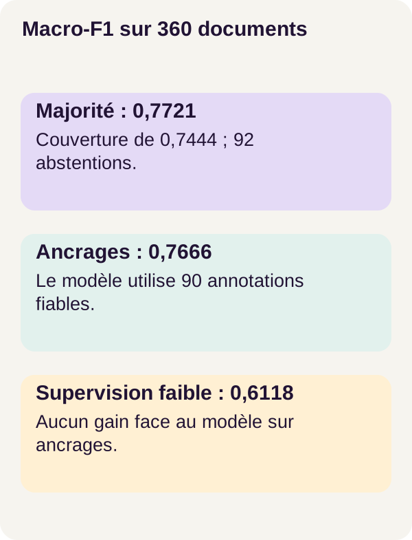
The methods do not share the same coverage: majority voting abstains on 92 documents.
What we have learned
A rule provides a partial opinion. It may be right, wrong or abstain. Abstention must not become a default business class, and a conflict must not be hidden to produce an answer at any cost.
EM estimates a hidden class using assumptions about votes. Anchors give it reliable reference points, but distributions with little information remain a limited training signal for the next classifier.
Finally, coverage, macro-F1 and probabilistic errors tell us different things. The workflow teaches us both to build a weak supervision pipeline and to recognize when it does no better than the reliable annotations already available.
Exercise: is a copied rule new information?
Before running the experiment, write down your hypothesis: what happens if we copy the ‘approved in the title’ rule? Does the vote count change? Have we learned anything new about the document? Predict the effect on the latent model and the text classifier separately.
To help you reason, return to the teaching example [2, 1, -1]. Duplicating the first opinion gives [2, 1, -1, 2]. Majority voting no longer sees a tie, although no new information has been observed. Two copies of the same condition remain dependent, even if they occupy separate columns.
The supplied variant duplicates this rule, retrains the affected pipeline and evaluates it on the same documents.
docker compose run --rm learning python -m ged_supervision_faible_statuts.cli exercise --config configs/minimum.yaml
docker compose run --rm inference python -m ged_supervision_faible_statuts.cli predict --config configs/minimum.yaml --variant duplicate
docker compose run --rm tutorial python -m ged_supervision_faible_statuts.cli evaluate-exercise --config configs/minimum.yaml
Open outputs/exercise-comparison.json and compare the measurements with your predictions. In the reference workflow, the latent model’s macro-F1 falls by approximately 0.2122, while the classifier’s rises by approximately 0.0144. These are score differences, not relative percentage changes.
The classifier’s Brier score increases slightly: its macro-F1 improvement therefore does not come with an improvement in this probabilistic measure. The copy provided no independent observation, and its effects are not identical at the two pipeline stages.
Do not take away a simplistic rule such as ‘duplication always lowers every score’. Instead, remember the question to ask: what information was actually added, and at which stage do we observe its effect?
For your own experiment, then choose a single rule and modify how it handles a negation. First write down what should change. Rerun the workflow in a separate extraction, retaining the same evaluation sets, then compare votes, abstentions, examples and metrics.
This personal modification is separate from the reference variant: its result is not known in advance. In a development workflow, use validation to choose an improvement and keep the final test separate from those choices, rather than continually tuning rules to improve its score.
Inspect the figures and check the files
Generate figures from your outputs, then check the checkpoints.
docker compose run --rm tutorial python lesson/figures/plot.py
docker compose run --rm tutorial python scripts/check_checkpoints.py
The files outputs/rules.json, outputs/evaluation.json and the figures let you work back from averages to examples. For V-033, follow the same path as the program: the clues in the document, rule opinions, estimated distributions, then classifier suggestions. An average result does not replace inspection of this path.
Negative tests check that the program rejects inconsistent input. They cover votes outside permitted classes, non-finite probabilities, incorrectly normalized distributions and invalid anchors, among other cases. Test success then means observing the expected rejection, not obtaining a class at any cost.
Troubleshoot and clean up
Compose failing? Start with its configuration check, included in the first commands. Examine the error before blaming the model.
A training state already exists? Use a clean extraction rather than overwriting it. Mixing results from two attempts would make comparisons difficult to interpret.
A distribution is rejected? Inspect the inputs and how they were constructed. An incorrect sum, a negative or non-finite value reveals a problem to understand. Do not silently replace probabilities with an arbitrary class to pass the check.
Before cleanup, save useful figures and results. The following commands stop the project, delete only outputs/, then end the workflow. The corpus and checkpoints are retained.
docker compose down
docker compose run --rm tutorial python scripts/clean.py --outputs-only
docker compose down
From tutorial to real application
The synthetic corpus lets us study the mechanism; it does not represent every wording and practice in an organization. For an electronic document management application, or EDM, start with reliable annotations representative of the texts and how they evolve.
Measure correlations between rules, coverage, per-class errors and calibration on a separate set. A rule exploiting a writing habit or a date may stop being useful when practices change. Titles, quotations and dates must not become proof of an administrative status.
On the application side, clearly distinguish the model’s suggestion from the official state. A screen could present the suggested opinion, the evidence used and an option for human review; this interface is an integration idea, not a feature already provided by the tutorial.
Add access rights, confidentiality, rule versioning, suggestion traceability, service monitoring and human oversight. These measures complement statistical evaluation: even a better score does not replace rules determining who can view a document or change its state.
Further exploration
Improve a rule based on identified errors. Choose an observable confusion, formulate a hypothesis, then measure whether the change reduces that error without simply shifting its cost to another class.
Compare several budgets for reliable annotations. The 90-anchor result provides a starting point for studying the effect of more or fewer verified examples. It does not let us predict the scores of those new experiments.
Examine dependencies between rules. Two rules can differ in code while almost always exploiting the same clue. The duplication exercise is a particularly visible case of this problem.
Build an interface for reviewing conflicting cases. It could display the document, votes, probabilities and human correction. The aim would be to make errors inspectable, not hide uncertainty behind a single label.
References for deeper explanations
The complete ZIP code describes the EM calculations and the reproducible R001 workflow. Links throughout the text point to Stanford’s introduction to weak supervision and to SciPy, PyTorch and scikit-learn documentation for numerical mechanisms and measurements.
These references supplement the explanations; they are neither a new validation of the project nor an invitation to replace its implementations. To reproduce the results, retain the ZIP’s dependencies, configurations and commands. The teaching examples of votes and probabilities are distinguished from corpus measurements.