





Imagine your web application's help center. A user reports that messages remain stuck in a queue after a worker stops. Your search engine finds an article explaining how to restart that worker. That is useful, but a second article describes how to replay messages whose processing has not been acknowledged. It also addresses the problem.
How can we teach the search engine to retrieve both procedures, without confusing them with other articles that use the same words but describe a different incident?
We will adapt an embedding model: the program that turns texts into vectors so they can be compared. The tricky part will not just be bringing a question closer to a good answer. We must also prevent a second good answer from accidentally becoming an example to push away during training.
Download the complete tutorial project
What we are building
The project builds a small search engine over a synthetic support corpus. It encodes queries and procedures using the same encoder, selects deceptively similar documents, then trains that encoder with a multi-positive contrastive loss. Finally, it saves the rankings and computes two metrics: Recall@5 and MRR@10.
In other words, we want to change what the model considers “close.” Two different procedures can be relevant to the same request; their difference alone should not make them incompatible competitors.
The walkthrough separates three responsibilities: annotations define the relevant procedures; training uses those annotations to adapt the model; evaluation then checks where the procedures appear in the results. The model does not define the right answers itself based on its preferences.
This program retrieves and ranks documents. It builds neither a complete RAG system—document retrieval followed by answer generation—nor a business rule that would decide how to resolve an incident automatically.
Concepts explained before the code
An embedding: coordinates for comparing texts
An embedding is a list of numbers computed from a text. You can imagine it as a point's coordinates: two texts whose vectors are close are considered similar by the model.
We do not manually choose a “failure” axis and a “restart” axis. The network's parameters, also called weights, determine how texts become coordinates. Adapting those parameters therefore changes the representation produced, without changing the procedures' text.
The model used is sentence-transformers/all-MiniLM-L6-v2, pinned to revision 1110a243fdf4706b3f48f1d95db1a4f5529b4d41 in locks/models.lock.json. Its official model card at that revision describes vectors with 384 coordinates. A document identifier lets you retrieve an article; its embedding is used to compare it with a query. The two are not interchangeable.
From text to a single vector
The computation involves several transformations. The tokenizer splits text into units, called tokens, then replaces them with numeric identifiers. A token can be a word or part of a word: it does not necessarily correspond to a space-separated word.
The Transformer then computes a vector for each position, taking context into account. We therefore have several vectors for one text, while search expects just one. Mean pooling combines them by computing a mean, coordinate by coordinate.
However, we must ignore padding: filler positions added so that several texts fit in an array of the same width. The attention mask indicates which positions are used, with 1 for those to retain and 0 for padding.
Take a two-coordinate teaching example, unrelated to the vectors actually produced by MiniLM. Two useful positions are [1, 2] and [5, 6]. A third position is padding. With a [1, 1, 0] mask, the mean is [(1 + 5) / 2, (2 + 6) / 2], or [3, 4]. The third position contributes neither to the sum nor to the denominator.
Normalizing: compare directions rather than magnitude
The walkthrough then applies F.normalize(..., dim=-1). This operation divides each vector by its norm, with protection for very small values. Here the norm is its geometric length: for [3, 4], it is sqrt(3² + 4²) = 5. The normalized vector therefore becomes [0.6, 0.8], whose norm is 1.
The dot product multiplies corresponding coordinates, then adds the results. For two vectors with norm 1, it equals their cosine similarity, a comparison of their directions. For example, [0.6, 0.8] compared with itself gives 0.6² + 0.8² = 1.
Without this normalization, a longer vector could obtain a higher dot product simply because of its magnitude. Here we want closeness of representation, not a length contest. The normalize documentation also explains how very small norms are handled.
A similarity score is not proof of business relevance. Two articles can discuss the same component without recommending the right action for the same incident.
Positives, negatives and misleading examples
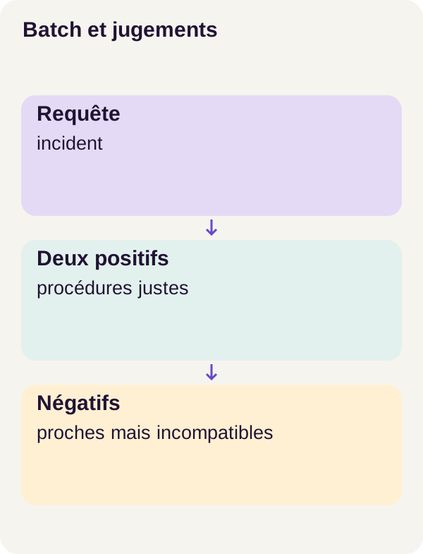
A positive is a document annotated as relevant to a query. A negative is used as a counterexample for that query. These roles depend on the request: a procedure may be relevant to one question but not another.
A hard negative is a counterexample that the model nevertheless scores highly. It lets us target a specific confusion. An article about the same message queue but a different problem can be more instructive than an article unrelated to queues.
Mining means selecting these counterexamples. It uses the model's ranking to find nearby candidates, but relies on annotations to exclude the right answers. The Sentence Transformers documentation on hard negatives presents this general principle; the tutorial retains its own selection code.
The danger is a false negative: a genuinely relevant procedure that training treats as incorrect. With two positives, a convention that recognized only one would create exactly this error.
Contrastive loss: learning through comparison
A loss is the number training seeks to reduce. A contrastive loss compares candidates: here, it encourages the model to give relevant documents more weight than the others.
Backpropagation computes gradients, which indicate how a change in parameters would change that loss. The optimizer uses this information to update the weights. The PyTorch tutorials on gradients and optimization detail this cycle. Computing embeddings with an already loaded model, without changing its weights, is instead inference.
Our adaptation starts from an existing model: we are not teaching it to read texts from scratch. We give it more precise supervision about the relationships expected in this corpus.
Temperature and softmax: adjusting the weight of differences
Softmax transforms a row of scores into positive numbers that sum to 1. It uses exp, the exponential function: an increasing function that yields a positive value even for a negative score. For candidate j, it computes exp(score_j) / sum(exp(scores)). These values express a distribution among the candidates considered, not a calibrated business probability. The PyTorch definition of softmax formalizes this operation.
During training, similarities are divided by a positive temperature before this computation. A low temperature accentuates differences; a higher temperature softens them.
For example, the fictional similarities [0.4, 0.2, 0, -0.2] become the scores [2, 1, 0, -1] after division by 0.2. The first candidate then receives approximately 64.39% of the softmax mass, compared with 32.92% at a temperature of 1. These are illustrative values, not the r1 settings or measurements. The ranking does not change under this positive division; the importance given to the differences changes.
Finally, log here denotes the natural logarithm, the inverse of the exponential function. logsumexp computes the logarithm of a sum of exponentials in a numerically stable way. We will use it to combine the contributions of several positives without naively computing very large exponentials. The torch.logsumexp documentation describes this operation.
Docker and GPU prerequisites
You should be able to read a Python function, work with lists and identifiers, and run commands in a terminal. The r1 walkthrough uses Linux x86_64, Docker Compose, NVIDIA Container Toolkit and a 24 GiB RTX 3090.
Also allow 16 GiB of RAM and 16 GiB of disk space, excluding shared Docker layers. RAM is the host's memory; graphics-card memory is VRAM. These provisions describe the project's setup, not proven minimums for every machine. No CPU profile is presented as a validated reproduction of the GPU walkthrough.
locks/models.lock.json pins the model assets and locks/environment.lock.json the expected environment. Keep these locks to reproduce the experiment: replacing a revision with the current branch would change the elements we are comparing.
The acquire service is the only one that downloads model assets. The gpu service then performs local computations. Building a Docker image and acquiring weights are two different operations: weights are the model's parameters, not the Python code that uses them.
The environment check initializes CUDA and performs a computation inside the container. Seeing the card from Linux is not enough. The documentation for Docker Compose GPU support and NVIDIA Container Toolkit explains this integration.
Data and core functions
Know the right answers before training
The synthetic corpus contains 240 documents and 72 test queries. Each query has exactly two positive_ids. These identifiers provide the reference used to determine which procedures are relevant.
Families are separated into train, validation and test before training. Train supplies the examples that affect the weights; validation is used to observe training choices; test remains reserved for the final ranking. Splitting families prevents a mere rephrasing of the same set of cases from appearing on both sides of the evaluation.
A training query mines only training documents. Mining ranks them with the current model, explicitly removes both positive IDs, then retains the negatives. It therefore does not guess their relevance. This boundary prevents a test procedure from already being seen by the optimizer as a counterexample.
Do not confuse the 240 documents reported for the corpus with the population eligible for training mining: the latter is restricted to the train split. Detailed counts and membership can be read in the prepared data.
Our running example: two procedures, not two copies
The r1 example atlas-queue-q0 contains this question:
The Atlas messages remain pending after the queue worker crashes. What should the operator do?
In other words, Atlas messages are still waiting after the queue worker crashes, and the operator needs to know what to do. This explanation accompanies the reading; it does not replace the experiment's original text above.
A worker is the process that handles jobs from a queue. An unacknowledged message has not received the expected confirmation that it was processed. Replaying such a message requires controlling repetition: an idempotency key identifies an operation so that replaying it does not improperly repeat its effects.
The two annotated procedures address distinct aspects of this incident:
| Positive identifier | Role of the procedure in this example |
|---|---|
atlas-queue-procedure-a |
Inspect and restart the worker. |
atlas-queue-procedure-b |
Replay unacknowledged messages with idempotency keys. |
We do not seek to merge these texts or assume that one always replaces the other. Both must remain positives for this query. Retrieving these articles does not, by itself, operationally validate their execution.
Build the mask from identifiers
A batch groups several examples processed together. The scores matrix contains one row per query and one column per candidate document. Its shape is therefore B × D, with B queries and D documents.
positive_mask has exactly the same shape. It contains True when the column's document is relevant to the row's query. A single row can therefore contain several True values.
The make_batch function in src/contrastive_search/mining.py builds this mask from identifiers, then checks that there are two positives per query. This is equivalent to a key-based join in an application: changing the order of rows must not change their meaning.
A diagonal marks only the positions where the row number equals the column number. By itself, it cannot represent two positives on one row. A batch-position convention must therefore not replace our annotations.
Reading the core of the loss
Here is the central, continuous excerpt from src/contrastive_search/losses.py. It receives already computed scores, a relevance mask and, optionally, a mask of candidates included in the calculation.
def multi_positive_nce(scores, positive_mask, allowed=None):
    if scores.ndim != 2 or positive_mask.shape != scores.shape:
        raise ValueError("B x D scores and positive mask required")
    allowed = (
        torch.ones_like(positive_mask, dtype=torch.bool) if allowed is None else allowed
    )
    if not torch.isfinite(scores).all():
        raise ValueError("Non-finite scores")
    if ((positive_mask & allowed).sum(1) == 0).any():
        raise ValueError("Each query needs an allowed positive")
    denominator = torch.logsumexp(scores.masked_fill(~allowed, -torch.inf), dim=1)
    numerator = torch.logsumexp(
        scores.masked_fill(~(positive_mask & allowed), -torch.inf), dim=1
    )
    return (denominator - numerator).mean()
Let's start with the inputs. scores is a PyTorch array of numbers, also called a tensor. positive_mask is its corresponding boolean array. When allowed is not supplied, all candidates are included.
Here, the name allowed means “included in the formula.” This mask is neither authentication nor a document-permissions rule. On these boolean arrays, ~ inverts True and False, while & applies an elementwise “and.”
The denominator considers all included candidates. masked_fill(~allowed, -torch.inf) replaces excluded scores with negative infinity. Since their exponential is zero, they no longer contribute to the sum. dim=1 requests this calculation across columns, separately for each query.
The numerator considers all included positives. The expression positive_mask & allowed retains the intersection of the two masks. Both correct procedures therefore contribute together to the numerator, rather than keeping just one.
For one query, we therefore compute:
L = log(sum of exp(scores) for included candidates) − log(sum of exp(scores) for included positives).
In the code, the names denominator and numerator refer to the logarithms of those two sums. Their difference equals −log(numerator / denominator). The final .mean() averages this loss across queries in the batch, not across positive documents taken separately.
Work through a calculation by hand
Return to the demonstration row [2, 1, 0, -1], with the first two documents positive and all candidates included. These four scores are illustrative; they are not captured model outputs.
| Column | Score | Positive document? | Rounded exp(score) contribution |
|---|---|---|---|
| 0 | 2 | Yes | 7.389056 |
| 1 | 1 | Yes | 2.718282 |
| 2 | 0 | No | 1.000000 |
| 3 | −1 | No | 0.367879 |
The sum of all contributions is approximately 11.475217. The sum for the two positives is approximately 10.107338. Their ratio is therefore approximately 0.880797, and the loss −log(0.880797) is approximately 0.126928.
Here, the model assigns approximately 88.08% of the softmax mass to the set of correct answers. The loss decreases as that mass approaches 1. The numerical calculations above are performed before rounding the displayed values.
With a mask declaring only column 0 positive, the numerator would retain only 7.389056. The loss would become approximately 0.440190. More importantly, column 1 would remain in the denominator without contributing to the numerator: increasing its score would increase the loss, even though its procedure is relevant. We will check the sign of its gradient in the exercise.
What this formula guarantees, and what it does not
The function avoids treating the second positive as a negative. However, it favors the set of positives, without requiring them to receive the same score. It is not an average of two independent losses, each requiring its own document to win alone.
One correct procedure can therefore receive most of the softmax mass, and the other much less. If all included candidates are positive, the numerator and denominator even become identical: the loss is zero regardless of their order.
That explains why we subsequently measure whether both procedures appear in the top 5. A low loss is not enough to demonstrate that each one is well ranked.
The safeguards also have a precise scope. The function checks the shape of scores and positive_mask, whether scores are finite and whether every query has at least one included positive. It does not itself check that there are exactly two: that check belongs to make_batch. The caller must supply compatible boolean masks.
The finite-value check occurs before masking. A NaN or infinity already present in scores is therefore rejected even if its column would later be excluded. The negative infinities deliberately introduced by masked_fill, by contrast, remove contributions from the calculation.
Finally, this excerpt does not encode texts, select negatives or divide similarities by the temperature. Nor does it contain a backward() call or a weight update. It computes a differentiable loss that the training loop then uses.
Install, check, then prepare the data
Extract the ZIP and move to its root directory. All the following commands run from that root, in the order shown.
First we prepare the directories, check the Compose configuration, build the images, acquire the locked assets, check CUDA and run the tests. The following six commands are the first six commands of the r1 walkthrough.
sh scripts/setup.sh
docker compose config --quiet
docker compose build acquire gpu
docker compose run --rm acquire python scripts/acquire.py --config configs/minimum.yaml
docker compose run --rm gpu python scripts/check_environment.py --config configs/minimum.yaml
docker compose run --rm gpu python -m pytest -q
docker compose config --quiet checks the configuration without displaying the entire resolved file. The build prepares the images. Acquisition validates the files defined by the locks; the environment check verifies CUDA computation; pytest runs the project's tests. The Docker Compose documentation details the validation command.
Do not continue if a step fails. A passing test suite checks program behavior; it does not yet tell us whether the adapted encoder will rank procedures better.
Now let's prepare the corpus, inspect the vectors and extract the negatives. We are not training the model yet.
docker compose run --rm gpu python -m contrastive_search.cli prepare --config configs/minimum.yaml
docker compose run --rm gpu python -m contrastive_search.cli inspect-embeddings --config configs/minimum.yaml
docker compose run --rm gpu python -m contrastive_search.cli mine --config configs/minimum.yaml
docker compose run --rm gpu python -m contrastive_search.cli check-loss --config configs/minimum.yaml
After prepare, inspect the splits and identifiers. After inspect-embeddings, relate the vectors to their source texts: an array of coordinates is not a complete ranking by itself.
After mine, open outputs/mining-audit.json. Check that the negatives come from train and that none of the positive_ids were selected as negatives. The expected false-negative fraction is zero relative to the known annotations. This check could not discover a third relevant procedure that nobody had annotated.
Finally, check-loss checks the formula on known tensors. It is used to detect a mechanism error before searching for it among thousands of training computations.
Train and check resumption
We will compare three training runs. The hard reference, launched without a variant option, uses hard negatives. random varies their selection; temperature varies the temperature. Each variant changes one experimental decision so that differences remain interpretable.
Mind the terminology: later, baseline will mean the model before this adaptation. The hard reference, on the other hand, is a training run. These are not two names for the same state.
The exact temperature values and other training settings remain those in the project's configuration. The numbers used in our calculation examples do not replace them.
The final commands trigger an interruption, resume from the checkpoint created and compare the resumed run. Keep this order: the file artifacts/checkpoints/interrupted/state.pt must exist before the command that loads it.
docker compose run --rm gpu python -m contrastive_search.cli train --config configs/minimum.yaml
docker compose run --rm gpu python -m contrastive_search.cli train --config configs/minimum.yaml --variant random
docker compose run --rm gpu python -m contrastive_search.cli train --config configs/minimum.yaml --variant temperature
docker compose run --rm gpu python -m contrastive_search.cli train --config configs/minimum.yaml --stop-after 10 --run-name interrupted
docker compose run --rm gpu python -m contrastive_search.cli train --config configs/minimum.yaml --resume artifacts/checkpoints/interrupted/state.pt --run-name resumed
docker compose run --rm gpu python -m contrastive_search.cli compare-resume --config configs/minimum.yaml
A checkpoint saves a computation's state. Recovering weights to perform a search and recovering the state needed to continue learning are two different needs. Depending on the loop, resumption may also depend on the optimizer, progress through the data and random generators. The PyTorch documentation on checkpoints for resuming explains why saving weights alone is not always enough. The exact contents of this project's checkpoint can be inspected in the archive.
compare-resume is precisely intended to check that the necessary state has been reconstructed, rather than judge how similar two curves look. Read its checks: loading without errors is not, by itself, proof of equivalent resumption.
Measure before the exercise
Now let's compute the reference rankings before making any guided changes in the exercise.
docker compose run --rm gpu python -m contrastive_search.cli evaluate --config configs/minimum.yaml
The command writes metrics and ranks to outputs/. These two output types complement each other: a metric summarizes the batch, while a ranking lets you understand what happened for a particular query.
For an initial reading, find a question's ID, its two positive_ids, then their positions in each ranking. Next, move on to averages over the test set. One successful search is not enough to establish the quality of the whole system.
Metrics before measurements
Recall@5: did we retrieve both procedures?
Recall@5, or recall at five results, is the fraction of relevant documents present among the top five:
Recall@5 = number of positives in the top 5 / total number of expected positives.
With two relevant procedures, only one in the top 5 gives 1 / 2 = 0.5. Both give 2 / 2 = 1. The final average combines the queries' contributions.
Here the denominator is 2, not 5. Recall asks “what proportion of the correct procedures did I retrieve?” It does not ask “what proportion of the five results is relevant?”, which would be a different metric, precision. Two correct procedures among five results can therefore yield 100% recall without all five results being relevant.
MRR@10: where does the first correct procedure appear?
For one query, the reciprocal rank is the inverse of the rank of the first positive within the top ten positions. A positive at rank 1 gives 1; at rank 2, 1 / 2 = 0.5; at rank 4, 1 / 4 = 0.25. If there is none in the top ten, the contribution is 0.
MRR stands for Mean Reciprocal Rank: we then average these contributions across queries. For example, three contributions of 1, 0.5 and 0 give an MRR of (1 + 0.5 + 0) / 3 = 0.5. This small calculation illustrates the metric, not the r1 batch.
MRR ignores the second positive's position once it finds the first. It must therefore be read alongside Recall@5, not instead of it. The Sentence Transformers retrieval evaluation documentation places these metrics in a setup based on queries, a corpus and annotations.
Six rankings to distinguish the two questions
Here are teaching examples with exactly two positives. The numbers indicate their ranks, starting at 1; the other documents are not relevant.
| Ranks of the two positives | Query Recall@5 | Reciprocal rank at 10 | What we observe |
|---|---|---|---|
| 1 and 2 | 1 | 1 | Both procedures are at the top. |
| 1 and 5 | 1 | 1 | Same metrics, but the second positive is lower. |
| 2 and 4 | 1 | 0.5 | Both are retrieved; neither comes first. |
| 1 and 8 | 0.5 | 1 | The first is ideally placed; the second is missing from the top 5. |
| 6 and 9 | 0 | Approximately 0.1667 | The positives are in the top 10, not the top 5. |
| 11 and 12 | 0 | 0 | No positive within the measured ranges. |
Two consequences become clear. Perfect Recall@5 can coexist with an MRR that still has room to improve. And even when both metrics equal 1, they do not prove that the two procedures occupy the first two positions.
Actual results and what we learned
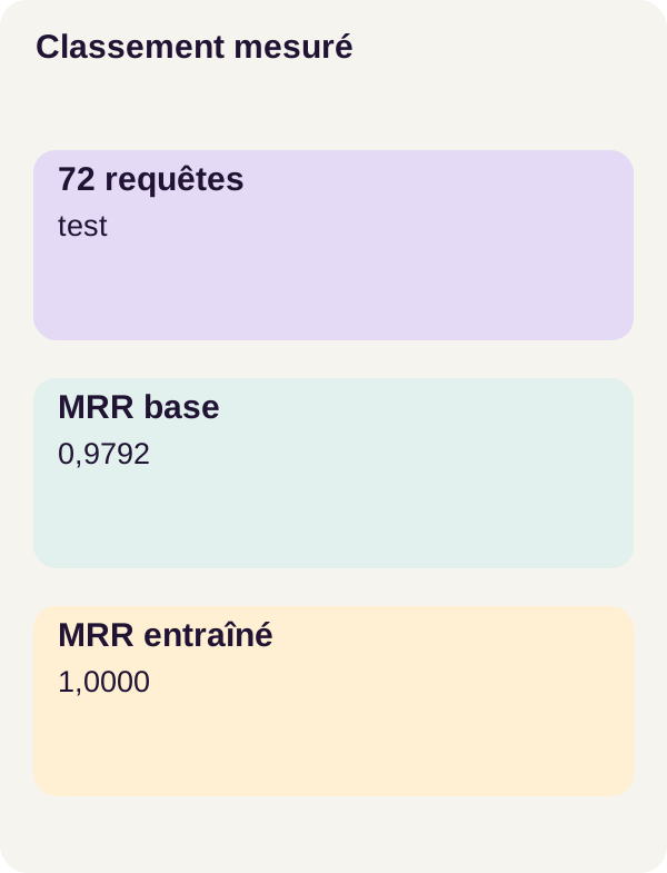
The following values are the r1 measurements reported on 72 test queries and 240 documents. They are distinct from the previous calculation examples.
| Evaluated state | Recall@5 | MRR@10 |
|---|---|---|
| Baseline, before adaptation | 1.0 | 0.9791666666666666 |
random training |
1.0 | 1.0 |
hard training |
1.0 | 1.0 |
temperature training |
1.0 | 1.0 |
The first observation is that recall does not improve: it is already perfect before training. The baseline retrieves both relevant procedures within the top five results for every evaluated query.
MRR, meanwhile, rises from 0.9791666666666666 to 1.0. After each of the three training runs, the first relevant procedure therefore ranks first for every query in the batch. This does not imply that the second always occupies rank 2: the teaching table above shows why.
All three trained variants obtain the same metrics. We therefore cannot claim a superiority for hard negatives that this table does not show. The synthetic corpus is small and already easy; it exposes how this protocol works, not a universal ranking of training strategies.
Nor does the aggregate provide the detailed distribution of baseline ranks. To find out which queries changed, reread the saved rankings rather than reconstructing a story from the average alone.
The main lesson is structural: relevance labels must survive batch construction. A second correct procedure remains correct, whatever its column in the matrix. And a correctly computed loss never removes the need to measure the final ranking.
Exercise: predict, then run
Return to the row [2, 1, 0, -1]. Columns 0 and 1 correspond to the two relevant procedures. Now imagine a diagonal-based mask retaining only one: only column 0 remains marked positive.
Before running the command, write down your prediction: will the gradient of column 1's score encourage that score to rise or fall?
To read the sign, keep a basic update in mind: new_score = score − step × gradient, with a positive step. A negative gradient therefore pushes the score up; a positive gradient pushes it down. Here we are discussing the derivative with respect to the score to isolate the mechanism.
docker compose run --rm gpu python -m contrastive_search.cli exercise --config configs/exercise.yaml
The exercise output retains both gradients and confirms the unjustified repulsion when the second positive is no longer marked. Compare it with your prediction.
To accompany that reading, here are the derivatives computed on our teaching row, with all candidates included and a single query. They are not presented as a capture from r1 training.
| Column | Gradient with two positives | Gradient with only the first positive | Effect of the second convention |
|---|---|---|---|
| 0, positive | −0.087144 | −0.356086 | The first positive is still encouraged. |
| 1, positive | −0.032059 | +0.236883 | The second positive is now pushed away. |
| 2, negative | +0.087144 | +0.087144 | The negative is still pushed away. |
| 3, negative | +0.032059 | +0.032059 | The negative is still pushed away. |
The sign change in column 1 is the flaw to remember. The model has not discovered that the procedure is incorrect: we gave it incorrect supervision.
In the actual network, scores share the same parameters. These derivatives describe the pressure the loss exerts on each score; they do not guarantee that each score will change independently in that direction after all weights are updated.
Then finish the artifacts and shut down the walkthrough, in this order:
docker compose run --rm gpu python lesson/figures/plot.py
docker compose run --rm gpu python scripts/check_checkpoints.py
docker compose run --rm gpu python scripts/clean.py --scope generated --dry-run
docker compose down --remove-orphans
The first command generates figures; the second checks checkpoints, including those created during training. clean.py --dry-run only previews cleanup and deletes no files. The last command stops the project's Compose resources. Do not confuse this preview with actually stopping the containers.
Adaptation, production, troubleshooting and cleanup
From the synthetic corpus to your documents
To adapt the mechanism, start with reviewed, versioned relevance judgments. A request can have two correct procedures, but also one, more than two or none. The “exactly two positives” contract belongs to this tutorial; it must not become an implicit assumption about your real data.
Keep training, validation and testing clearly separated. Analyze false positives by family: these are procedures ranked as useful even though they do not address the request. Distinguish them from mining false negatives, which are correct procedures wrongly used as training counterexamples.
A hard negative may be an unannotated relevant document. The absence of its ID from the positives list does not prove that it is useless. Keep the mining audit and a review mechanism. Correcting annotations is a data decision, not an automatic effect of the model.
If you adapt the model, also recompute document representations with the corresponding encoder before comparing new queries: mixing two encoder states no longer reproduces the same-model search described here. This consistency follows from how the walkthrough works; it is not an index-migration feature already provided.
The Atlas question shown above is in English, and the model card indicates language: en. A French corpus therefore constitutes a separate experiment to evaluate; the article's explanatory French translation does not validate its quality in French.
Do not turn a local average into a service promise
Measure latency under your target load. A warm per-query measurement—when the model is already loaded—describes neither concurrent traffic nor waiting in a request queue. It also does not validate an ANN index, meaning approximate nearest-neighbor search used to avoid exhaustively comparing all vectors.
The project does not become a production API because Recall@5 equals 1. Document ingestion, access permissions, index updates, backups, input limits and observability require application-specific design and testing. These extensions are separate from the measured experiment.
Diagnose without silently changing the experiment
CUDA fails. First rerun check_environment.py and consult the NVIDIA Container Toolkit guide. A GPU access error is not a reason to change the loss formula.
Acquisition fails. Check the acquire service's network, then rerun the same command. Do not modify locked files to make a different asset acceptable.
The loss rejects a query with no included positive. Inspect the IDs, the split and the intersection positive_mask & allowed. Removing the check would eliminate the symptom, not the lack of supervision.
The scores are surprising. Examine the ranks of both positives, not just the first result or the loss. Perfect MRR can hide a second positive ranked too low; already perfect Recall@5 cannot increase further.
Finally, docker compose down --remove-orphans stops the project's services and retains the local files described by the walkthrough. clean.py --dry-run only shows what it would target. Keep reference outputs before any separate experiment or actual deletion.
Official sources
Model and learning. The all-MiniLM-L6-v2 model card presents the model; its locked version is linked above. The Sentence Transformers documentation on losses, hard-negative mining and retrieval evaluation explores these topics further. It does not replace the multi-positive formula specific to this archive's code.
Numerical computation. The PyTorch references for normalize, softmax and logsumexp explain the operations used in the explanations. The PyTorch versions page serves as an installation reference; to reproduce r1, keep the environment fixed by the project's locks.
Environment. Consult Docker Compose GPU access and the NVIDIA Container Toolkit guide to understand the integration between host, container and graphics card.