





Imagine a back-office activity log: a document is imported, indexed, assigned to a team, then sent for review. Most cases follow fairly regular paths. But some skip a stage, go through revision several times or take much longer to move forward.
You could write a series of conditions to detect them. But how can you distinguish a truly unusual path from a normal variant your rules did not anticipate? And what happens if the team changes how it works?
We will build a detector that learns to predict the next event and its delay, then compares that prediction with what actually happens. When sufficiently surprised, it flags the case for review. It decides neither that someone committed a fault nor that a document is noncompliant.
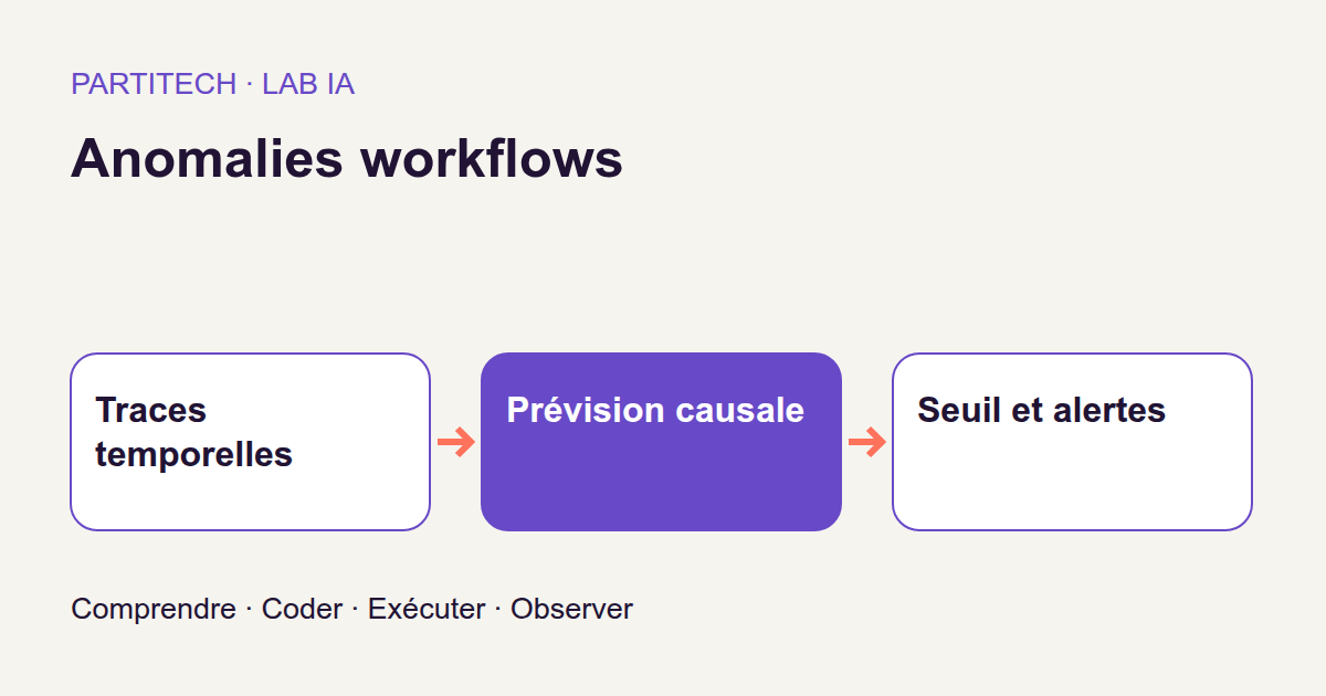
The workflow is concrete: event log → observed prefix → prediction → surprise measurement → threshold → alert to review. We will train a small recurrent network, compare it with two simple methods and test its response to a new yet acceptable practice.
The model receives neither identities, case families nor absolute timestamps. Data is synthetic: it enables a controlled experiment, not measurement of incident frequency in a company. The small calculations throughout the article are teaching examples; r004 reference results are presented separately.
Download the complete project, revision r004
Define an anomaly as surprise, not noncompliance
Read a trace like an application log
EDM, or electronic document management, retains documents and their operations. A workflow is their path through stages. A trace is the ordered event sequence for one case; a prefix is the beginning of that sequence up to a given position.
The project vocabulary contains eight events: IMPORT, INDEXATION, AFFECTATION, REVUE, REVISION, APPROBATION, PUBLICATION and ARCHIVAGE. Four fictional roles identify the role associated with an event without providing an individual identity.
Take this illustrative prefix: IMPORT → INDEXATION → AFFECTATION → REVUE. At this point, we know review occurred. We do not yet know whether the next stage will be revision or approval, or how long it will take.
A normal simulator trace may include REVISION → REVUE and may omit publication. Not every loop or absent stage should therefore be treated as an error. Injected perturbations—skipping, looping, permutation and extended delay—test the detector within this corpus. They do not define a universal document policy.
Separate learning, tuning and measuring
The model learns normal paths on the training set, called train. The validation set here fixes the alert threshold. The test then measures the resulting rule without readjusting the threshold to improve figures.
The populations explicitly described in the protocol are:
| Set | Normal traces | Explicitly counted perturbed traces |
|---|---|---|
| Training | 840 | None in the described training |
| Validation used for threshold | 90 | Not used to select the threshold |
| Test | 90 | 90 |
A caution about the overall count. The corpus is described as 120 families of ten traces, totaling 1,200 traces. Explicit counts above total 1,110. The supplied description does not specify where the remaining 90 belong: this needs checking in corpus generation. We retain reported training, calibration and test populations without filling the gap through an assumed allocation.
Separation also respects time: training precedes validation, which precedes testing. Each family has its own time window. Cases, traces and windows do not cross sets, also called splits.
This does not mean symbol sequences are entirely different. A beginning such as IMPORT → INDEXATION may appear everywhere. With only eight events, prohibiting every shared prefix would create an artificial problem. Cases and their windows must remain separate, not the vocabulary needed to describe activity.
Reject invalid source data before looking for anomalies
The program distinguishes malformed data from an infrequent event. A negative duration, unknown event type or duplicated source order invalidates input before statistical calculation.
Equal timestamps are allowed. Source order, which breaks event ties, then determines their sequence. A zero delay is therefore a valid observation, not an automatic anomaly.
The stream is checked for nondecreasing order before stable sorting. Why this order of operations? Suppose an export shows 10:05 followed by 10:02. Sorting rows immediately would yield an apparently clean chronology while hiding source inconsistency. The workflow prefers flagging the issue rather than turning it into statistical surprise.
What the model knows at each instant
At the current position, it receives three pieces of information: the event, its role and the delay already elapsed since the previous event. This delay is transformed into log1p(delay) / 10.
log1p(x) computes the natural logarithm of 1 + x. The logarithm compresses large values; adding 1 also makes zero delay usable. With illustrative durations of 9, 99 and 999 seconds, the temporal input is approximately 0.2303, 0.4605 and 0.6908, respectively. The network therefore does not directly receive 9, 99 and 999. The torch.log1p documentation details this calculation.
Watch the shift: the input delay concerns the past; the predicted delay concerns the next stage. The model receives neither that next event, its role, perturbation type, case ID, family nor absolute time. Future events serve as training targets, not inputs at the same position.
An alert on this transition can be calculated only after the next event arrives. If it arrives after a long wait, the program can then compare observed delay with its prediction. However, this workflow provides no alarm during an ongoing wait. That would require an additional mechanism to design and evaluate.
Here, causal means ‘without reading the future’. It does not mean ‘able to explain the business cause’. A test modifies a future suffix—the end of the trace—and checks that raw scores for the unchanged prefix do not change.
The causal model and its two heads
A small state that moves forward with the case
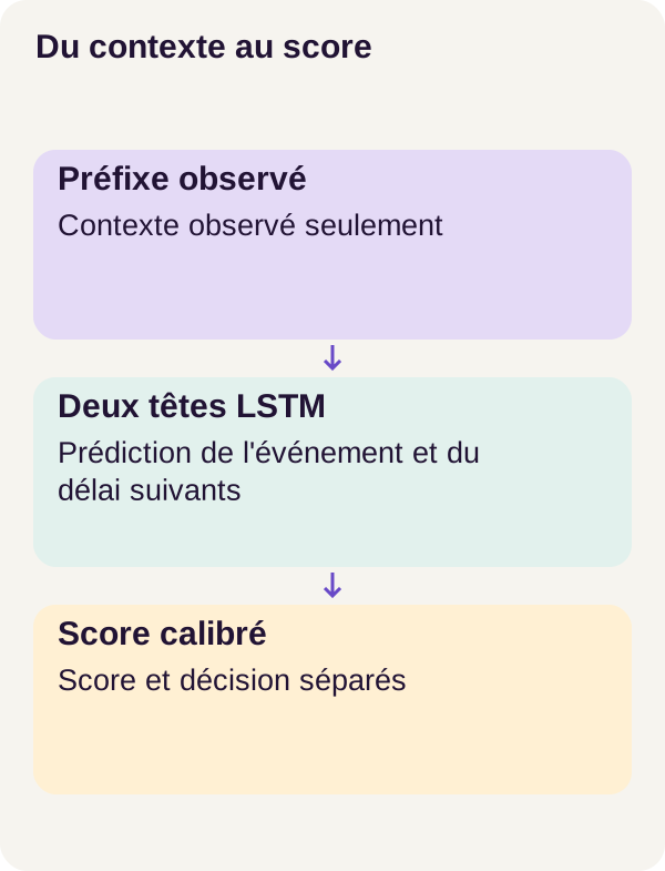
An LSTM, short for Long Short-Term Memory, processes a sequence in order and updates a numerical state at each position. Imagine a function traversing an event array while retaining a summary of what it read. Here, how that summary is built is learned rather than written as conditions.
The project’s LSTM is unidirectional, with 64 units. It reads only forward. Its state starts at zero for each case: the previous case’s summary does not become the next case’s context. Internal mechanisms and states are described in the PyTorch 2.8 documentation.
Before reading, categories become vectors. An embedding here is a row in a learned number table: each event gets 16 values, each role 8. This is not linguistic understanding of the word REVUE, but learning a useful representation of its category. The Embedding documentation describes this lookup-table principle.
Adding the temporal value gives 16 + 8 + 1 = 25 numbers per position. The LSTM transforms them into a 64-value state. Two heads, meaning small output layers, use that state: one predicts the next event, the other the next delay’s parameters.
Follow dimensions through the code
Here is the first project excerpt, retained unchanged:
import torch
from torch import nn
import torch.nn.functional as F
from .events import make_prefix_targets


class SequenceModel(nn.Module):
    def __init__(self):
        super().__init__()
        self.events = nn.Embedding(8, 16)
        self.roles = nn.Embedding(4, 8)
        self.lstm = nn.LSTM(25, 64, batch_first=True)
        self.event_head = nn.Linear(64, 8)
        self.delay_head = nn.Linear(64, 2)

    def forward(self, event, role, previous):
        x = torch.cat(
            [self.events(event), self.roles(role), previous.unsqueeze(-1)], -1
        )
        # No state argument: every batch starts fresh, no state crosses cases.
        hidden, _ = self.lstm(x)
        logits = self.event_head(hidden)
        parameters = self.delay_head(hidden)
        return logits, parameters[..., 0], F.softplus(parameters[..., 1]) + 0.001
A tensor is a numerical array with potentially multiple axes. To read this code, call the number of traces in a batch B and the number of positions after padding T. Event and role names are converted into integer identifiers; event, role and previous each have shape [B, T].
self.events(event) returns [B, T, 16], and self.roles(role) returns [B, T, 8]. previous.unsqueeze(-1) adds a delay axis to obtain [B, T, 1]. Finally, torch.cat(..., -1) joins the three blocks along the last axis, giving [B, T, 25].
batch_first=True means the first axis denotes the batch. hidden then contains a 64-value state at every position, giving [B, T, 64], not just one final summary per trace. Passing no state to self.lstm(x) resets states on that call; the model does not automatically retain a session between calls.
The event_head produces [B, T, 8]: eight logits, or raw scores, for the eight events. These numbers are not yet probabilities. The delay_head produces [B, T, 2], whose components become mu and raw_sigma.
mu describes the center of the predicted distribution of log(1 + delay). sigma describes its spread as a standard deviation: a small value expresses a tighter temporal prediction.
The last line uses softplus(raw_sigma) + 0.001 to retain positive spread. Softplus is a smooth transformation based on log(1 + exp(x)); it lets the network learn without allowing a negative standard deviation. This constraint applies to sigma, not mu: the excerpt does not directly bound the delay obtained by converting mu back.
Learn the next event: penalize surprise
During training, the program knows which event follows each normal prefix. It asks the model to assign that event high probability. The loss function is the number training seeks to reduce.
For the event component, we use cross-entropy. With a categorical target, it corresponds to −log(probability of the event actually observed).
A teaching example: if the model assigns probability 0.8 to the event that occurs, its loss is approximately 0.2231. If it assigns only 0.05, loss is approximately 2.9957. The less likely the actual event was considered, the greater the surprise.
The code passes logits directly to F.cross_entropy, which performs the appropriate calculation. No prior softmax is needed in this excerpt. With reduction="none", we retain a loss per position instead of immediately obtaining an overall mean.
Learn delay without confusing its two scales
The temporal target is z = log(1 + next delay). This target is not divided by ten. Division by ten applied only to the previous-delay feature supplied as input.
The model approximates z with a Gaussian distribution, a bell curve centered on mu with standard deviation sigma. Temporal loss is calculated as:
NLL_delay = log(sigma) + (z − mu)² / (2 × sigma²)
NLL means negative log-likelihood. The squared term penalizes deviation between the target and predicted center relative to the stated spread. log(sigma) prevents indefinitely widening the spread at no cost. The Gaussian constant is omitted, as specified by the workflow. The GaussianNLLLoss documentation presents the general formula using variance; here, variance is sigma² and the calculation is written directly.
Take a numerical example separate from trained outputs: mu = log(11) and sigma = 0.5. An observed delay of 10 seconds gives z = mu, hence a loss of approximately −0.6931. A delay of 30 seconds gives approximately 1.4538. It is farther from the stated center and receives a larger penalty.
A negative temporal loss is not a negative probability. We work with a continuous density, not a category probability; density height can exceed 1, and the constant is removed here. Do not convert this NLL into a ‘risk percentage’.
The mask: do not learn from padding
Traces differ in length. To arrange them in a rectangular batch, padding is added on the right. The boolean mask indicates real positions with targets: True for useful positions, False for added ones.
Batch construction, located between the two excerpts in the source file, prepares tensors and this mask. The following function receives those data:
def components(logits, mu, sigma, targets, z, mask):
    if (
        mask.dtype != torch.bool
        or not mask.any(1).all()
        or ((mask[:, 1:] & ~mask[:, :-1]).any())
    ):
        raise ValueError("Nonempty real prefix mask required")
    # Select before calculating: a padded NaN target cannot contaminate loss.
    event = torch.zeros_like(mu)
    delay = torch.zeros_like(mu)
    event[mask] = F.cross_entropy(logits[mask], targets[mask], reduction="none")
    delay[mask] = torch.log(sigma[mask]) + (z[mask] - mu[mask]).square() / (
        2 * sigma[mask].square()
    )
    return event, delay
The first condition requires a boolean mask, at least one real position per trace and no return from False to True. Thus, [True, True, False, False] is valid, but [True, False, True, False] is rejected: real content must form a continuous prefix.
event and delay start at zero. Calculations then run only on elements selected by mask. The key is select before calculating, not calculate everywhere and multiply by zero afterward: NaN, an undefined numerical value, remains problematic even multiplied by zero. A NaN in a padding target must not contaminate real losses.
This function returns two loss arrays; it does not yet compute the final mean. The project loop first averages positions within each trace, then traces within the batch. A long trace therefore does not receive extra weight simply because it has more stages.
A teaching example: a two-position trace with loss 2 everywhere and an eight-position trace with loss 1 everywhere give a per-trace mean of (2 + 1) / 2 = 1.5. Averaged directly over ten positions, they would give (2 × 2 + 8 × 1) / 10 = 1.2. These are different weightings.
Visible checks concern the mask. They do not by themselves exhaustively validate every shape, value and spread one might pass directly to components().
Return to seconds: a median, not a mean
The workflow uses expm1(mu), meaning exp(mu) − 1, to return to a duration. Under this Gaussian approximation of z, this is a conditional median: it divides the predicted distribution in half, given the prefix. It is not its mean.
In our example with mu = log(11) and sigma = 0.5, the median is 10 seconds, while the transformed variable’s mean would be exp(mu + sigma² / 2) − 1, approximately 11.4646 seconds. The logarithmic transformation makes these summaries different. The SciPy lognormal documentation explores exponentiating a Gaussian; here we subtract 1 to recover delay.
Another nuance: published NLL is calculated in z space, not directly as a density in seconds. Changing variables in a density would require factor 1 / (1 + delay), called a Jacobian; its negative logarithm adds log(1 + delay) to NLL, along with the Gaussian constant for the full form. We do not make this change in the r004 score: modifying it would change the detector and calibration.
Why compare four methods?
The rules method encodes simulator transitions. It is an explicit reference with this knowledge of the generator, not a universal business policy.
The bigram counts transitions between consecutive events in train. It learns local frequency without retaining the entire prefix. Add-one smoothing adds a pseudocount to possibilities: a never-observed transition does not automatically receive zero probability. For example, with 12 outgoing transitions and eight possible successors, an absent successor would receive (0 + 1) / (12 + 8) = 0.05.
The event LSTM minimizes only cross-entropy. The joint LSTM minimizes cross-entropy plus 0.1 times delay NLL. All receive the same available prefixes, even if they use the information differently. The event LSTM notably retains the inputs described above: its name describes its training objective, not removal of past delay from input.
The 0.1 weight concerns training. Later, we encounter a 0.5 weight for constructing the alert score: these numbers have different roles.
Reproduce the complete workflow
Step 1 — prepare and verify computation inside Docker
You should be able to read Python, work with arrays and use a terminal with Docker. Probability and tensor concepts support the calculations just explained. The workflow uses FP32 on CUDA: 32-bit floating-point numbers computed on an NVIDIA GPU.
Extract the ZIP into a new folder and open a terminal at its root. All following commands run from this directory. Retain versions and resources specified by project files; article excerpts do not replace the complete environment.
sh scripts/preflight.sh
sh scripts/setup.sh
docker compose config --quiet
docker compose build acquisition tutorial learning inference calibration
docker compose run --rm acquisition python scripts/acquire.py --config configs/minimum.yaml
docker compose run --rm tutorial python scripts/check_environment.py
docker compose run --rm tutorial python -m pytest -q
Preflight checks Docker, GPU, memory and disk. setup.sh prepares the project environment; docker compose config --quiet checks configuration, then build builds services.
Here, acquisition downloads no pretrained model: locks/models.lock.json declares no external files. The network is initialized locally and trained on traces. This stage is retained to check workflow assets, not retrieve a large language model.
check_environment.py actually runs an LSTM and its gradients inside Docker. A GPU visible on the host is therefore insufficient. The gradient indicates how loss varies when parameters change, enabling training adjustments. pytest tests then check program behavior independently of detection metrics.
What to observe: each command must succeed before the next. Do not substitute GPU presence in Linux for failed computation inside the container.
Step 2 — prepare traces and inspect the mechanism
docker compose run --rm tutorial python -m ged_anomalies_workflows.cli prepare --config configs/minimum.yaml
docker compose run --rm inference python -m ged_anomalies_workflows.cli baseline --config configs/minimum.yaml
docker compose run --rm inference python -m ged_anomalies_workflows.cli inspect-mechanism --config configs/minimum.yaml
prepare builds the corpus. Locate reported populations, temporal splits and source checks, including the counting issue noted earlier. baseline supplies simple references; inspect-mechanism lets you examine calculations before full training.
Follow a prefix: what information is available, which event serves as target, and which interval does the delay describe? This reading avoids discovering only at the end that a column contained a future answer.
Step 3 — train, score and calibrate
sh scripts/train_variants.sh
docker compose run --rm inference python -m ged_anomalies_workflows.cli score --config configs/minimum.yaml
docker compose run --rm calibration python -m ged_anomalies_workflows.cli calibrate --config configs/minimum.yaml
docker compose run --rm tutorial python -m ged_anomalies_workflows.cli evaluate --config configs/minimum.yaml
train_variants.sh orchestrates both LSTM training runs. score applies models to prefixes. calibrate fixes thresholds on normal validation traces. Finally, evaluate measures results. The explanations below detail these outputs; retain them before running the exercise.
Training uses AdamW, with learning rate 0.003, weight decay 0.001, norm clipping 1, batches of 32 traces and 25 epochs. The protocol performs 27 updates per epoch. Both LSTMs share seed 17.
An epoch is one pass over the training set; a batch groups traces for a calculation. The optimizer adjusts parameters afterward. Learning rate sets update scale, and weight decay reduces weights according to AdamW. Norm clipping limits the norm of the gradient used: it does not mean ‘every weight must stay below 1’.
Verify resumption, not merely a similar score
The workflow compares continuous training for 25 epochs with interruption after ten followed by fifteen resumed epochs. A checkpoint saves the state needed to continue: model, optimizer, data sampling order (sampler), random generators (RNG) and history.
Reloading weights alone does not reproduce the continuation exactly. Likewise, two training runs finishing with the same recall are not necessarily identical. Resumption must restore protocol-specified states. The PyTorch reproducibility documentation also notes that numerical identity is not guaranteed after a platform or version change.
Local checkpoints are considered trusted states. The public audit reloads JSON weights and prefix outputs without loading an external pickle. This describes this workflow; do not substitute an arbitrarily downloaded checkpoint.
Calibrate a comparable score before testing
Put both components on a usable scale
We now have several surprise measurements, but not yet an alert rule. The rules method gives 0 or 1. The bigram and event LSTM use the observed event’s surprise.
For the joint LSTM, directly adding cross-entropy and delay NLL would make the result depend on their numerical scales. The project standardizes them separately, using only the mean and standard deviation computed on normal train prefixes:
standardized component = (value − train_mean) / train_standard_deviation
Subtract the usual level, then divide by the usual spread. A result of 2 means ‘two standard deviations above the training mean’, not ‘twice as dangerous’.
The joint score then adds the standardized components using the workflow’s fixed weight of 0.5. This weighting belongs to score construction, not the training loss weighted at 0.1.
A teaching example with fictional parameters: event surprise 1.4, mean 1 and standard deviation 0.2 give 2. Delay NLL 1.5, mean −0.5 and standard deviation 1 also give 2. Both components are now expressed relative to their usual spread. Applying weight 0.5 to a component of 2 reduces its contribution to 1. These calculations illustrate standardization and weighting; the executed combination remains the ZIP’s score command. Negative values are not erased before standardization.
A constant or non-finite component is rejected. Zero spread would prevent division; silently replacing the result with zero would hide the issue. Statistics are not recalculated on the test to make its scores more favorable.
From prefix to trace
A trace’s score is the maximum of its causal scores: one highly surprising transition can suffice. During progressive reading, this is the maximum of scores already calculable; the final score uses every observed prefix.
This choice has a simple consequence: a long trace offers more opportunities for a high score. Evaluation therefore retains length strata, groups of comparably sized traces. A good overall average could hide more false positives on long cases.
The 95% quantile: an exact rank, not a promise
Each method sorts scores from its 90 normal validation traces and retains the value at index ceil(0.95 × 90) − 1. ceil rounds upward: ceil(85.5) − 1 = 85. With zero-based indices, this is the 86th value in ascending order.
An alert then requires score > threshold. Equality does not alert. If all values were distinct, only the four after the 86th would exceed the validation threshold: 4 / 90 ≈ 4.44%. With ties, there may be fewer.
This detail prevents two misunderstandings. An empirical 95% quantile means neither ‘exactly 5% false positives’ nor ‘never more than 5% on future cases’. It defines a reproducible procedure on a given sample.
Validation anomalies are not used to choose this threshold. Testing follows. This calibration also does not turn the score into an incident probability: thresholds remain specific to each method’s scale. Changed practices or temporal dependencies may alter behavior.
Understand the metrics before the results
Precision, recall and false positives: three different questions
A correctly flagged perturbed trace is a true positive. A normal trace that alerts is a false positive. An unflagged perturbation is a false negative.
Take a small example: eight of ten perturbed traces alert; one normal trace also alerts. Precision is 8 / 9: among nine alerts, how many correspond to perturbations? Recall is 8 / 10: among ten perturbations, how many were detected?
The false positive rate, by contrast, divides flagged normal traces by all normal traces. It is not equal to 1 − precision, whose denominator is the number of alerts.
These measurements evaluate detection of generator-defined perturbations. They grade neither a case’s severity nor a person’s responsibility.
Average precision measures ranking, not one threshold
Average precision, or AP, examines what happens as the threshold descends through ranked scores. Each newly included group changes precision and recall. AP sums precisions weighted by recall gains: AP = sum(recall_gain × precision). The scikit-learn documentation gives this definition; it does not replace the ZIP evaluator or add a dependency.
Here, equal scores are handled together. Imagine just two traces with identical scores, one perturbed and one normal. No threshold can select the first without the second. Artificially placing the perturbation before the normal trace would improve apparent ranking without extra information.
AP of 1 and a false positive at the selected threshold can coexist. If every perturbation ranks above normal traces, ranking is perfect; a threshold previously fixed on validation may nevertheless be low enough to include a normal trace. We do not raise it after examining the test.
Two different meanings of delay
Delay prediction error is expressed here in seconds. It compares predicted duration with observed duration.
Detection delay, however, is expressed as the number of events after perturbation. A median of 0 means no additional event is needed for at least half the detected cases under this reference point. It means neither zero waiting seconds, zero computation milliseconds nor anticipation of the perturbation.
This median covers detected cases only. A method could quickly detect a few cases while missing many others, so it must be read alongside recall. Alerts before perturbation also deserve separate inspection rather than being treated as successful anticipation.
Results: a synthetic improvement to interpret cautiously
Decisions at the validation-fixed threshold
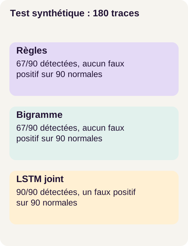
The test contains 90 normal and 90 perturbed traces. Perturbation prevalence is therefore 50%: an artificial prevalence, not a production observation.
Here are r004 counts and rates. Table false negatives are derived from 90 perturbations and published detections; rates are rounded to six decimal places.
On mobile, scroll the table horizontally.
| Method | Perturbations detected | Perturbations missed | False positives | Recall | Precision | False positive rate |
|---|---|---|---|---|---|---|
| Rules | 67/90 | 23 | 0/90 | 0.744444 | 1 | 0 |
| Bigram | 67/90 | 23 | 0/90 | 0.744444 | 1 | 0 |
| Event LSTM | 67/90 | 23 | 4/90 | 0.744444 | 0.943662 | 0.044444 |
| Joint event+delay LSTM | 90/90 | 0 | 1/90 | 1 | 0.989011 | 0.011111 |
The joint model finds every perturbation in this test with one false alert. Its precision is 90 / 91 = 0.989011, while its false positive rate is 1 / 90 = 0.011111. The event LSTM finds as many perturbations as simple methods but adds four false positives: its complexity delivers no gain on these decisions.
The joint model’s median detection delay is 0 events among detected cases. Each of the other three methods leaves 23 perturbations undetected after the change.
Ranking and prediction errors
Published thresholds and AP values follow. Thresholds must not be compared as a shared severity scale.
| Method | Threshold | Approximate average precision |
|---|---|---|
| Rules | 0 | 0.872222 |
| Bigram | 1.391023 | 0.887963 |
| Event LSTM | 1.386817 | 0.905482 |
| Joint event+delay LSTM | 4.284417 | 1 |
The rules case explains its AP. Score 1 groups 67 perturbations with no normal trace: precision is 1 and recall reaches 67 / 90. Adding the score-0 group includes the remaining 23 perturbations and 90 normal traces: precision becomes 0.5. AP is therefore 67 / 90 × 1 + 23 / 90 × 0.5 ≈ 0.872222. This is derived from published counts, not a new run.
Across 1,198 test prefixes, mean cross-entropy is 1.494473 for the event model and 1.290952 for the joint model. The joint model’s median absolute delay error is 8.026882 seconds. These measure predictions on this corpus; cross-entropy of 1.29 is not a proportion of 129%.
The joint model therefore improves detection in this experiment. However, the table does not detail the 23 perturbations other methods missed: alone, it does not establish that each is an extended delay.
Why 98.9% precision does not transfer to production
Perform a purely illustrative calculation, without assuming the model would retain performance on real cases. Among 10,000 traces with only 100 perturbations, imagine recall 1 and the same false positive rate of 1 / 90.
The system would flag all 100 perturbations, but also 9 900 / 90 = 110 normal traces. Precision would then be 100 / (100 + 110) ≈ 47.62%, not 98.9%.
Assumed rates have not changed; the population has. That is why balanced-test results alone cannot predict the workload of a human review queue.
Exercise: a new normal practice
Predict before running
The team now accepts a double REVISION → REVUE loop as normal practice. We neither retrain the model nor recalibrate the threshold. Can a network that rarely encountered this repetition still consider it suspicious? Must a rule checking only local transitions react the same way?
Write your hypothesis for all four methods, then run the exercise. Initial results and calibration are retained and hash-checked to prevent silent replacement.
docker compose run --rm tutorial python -m ged_anomalies_workflows.cli exercise --config configs/minimum.yaml
Compare with the workflow answer
The exercise’s 60 traces are now normal. Rules and bigram flag none. Both LSTMs flag all: 60 false positives out of 60, or 100% in this set.
This does not contradict the joint model’s good test score. The detector learned a certain frequency of paths; practice changed without changing training or threshold. A sequence can therefore be statistically unexpected and perfectly acceptable to the team.
Local transitions may already be permitted while their repetition in a longer history remains unusual to the sequence model. This is a mechanism-based interpretation to compare with outputs, not a complete causal explanation of every alert.
The exercise does not ask you to raise the threshold until alerts disappear. It asks you to qualify the new practice, create a new revision and plan a separate control set. Retraining or recalibration after that decision will be a new experiment whose result is not claimed here.
Then generate figures and check checkpoints before cleanup:
docker compose run --rm tutorial python lesson/figures/plot.py
docker compose run --rm tutorial python scripts/check_checkpoints.py
Troubleshoot, clean up and prepare production
Retain useful errors
If Docker does not make the GPU available, follow preflight diagnostics, then retry in a newly extracted folder. The environment check must successfully compute inside the container; host GPU status does not replace it.
If a trace is rejected for negative duration, unknown event or duplicated source order, inspect the export before the model. Do not bypass rejection with sorting that hides the original inconsistency.
If resumption differs from continuous execution, retain checkpoints for inspection. Compare restored states and versions rather than settling for a similar final score. Before deleting anything, save useful results and figures.
Clean up only what is intended
docker compose down
docker compose run --rm tutorial python scripts/clean.py --outputs-only
docker compose down
The first docker compose down stops project services. The script displays and deletes only outputs; the final shutdown ends the workflow. It removes no models, data, global volumes or other projects. No general Docker cleanup is required.
Workflow isolation has a precise scope
Services use a read-only root filesystem, no extra Linux capabilities, no-new-privileges, CPU, memory and process limits, and a temporary directory in tmpfs. Training, inference and calibration roles mount only resources necessary for their operations.
These restrictions limit available access and resources. They do not mean no output can be written: required locations are provided by role. Likewise, no third-party weight download does not mean image building is network-free: it may resolve dependencies defined in the build file. Model computations themselves are network-isolated.
This separation notably reduces accidental label-reading risks in the exercise. It is neither protection against a Docker administrator nor security certification.
Design an alert someone can handle
A real application should present the observed prefix, relevant event and delay, score, threshold and versions. This would let an operator understand what triggered the alert, without claiming the model explains the cause of delay or repetition. This interface is additional product work, not a feature already demonstrated here.
Real monitoring must also handle time zones, late arrivals, concurrent events and case identity. A total order convenient for a data table does not describe every causal relationship in a parallel workflow. If operations are simultaneous, ordering them by convention does not prove one caused another.
Authentication, permissions, filtering, APIs, a human review queue, model versioning, observability, load tests, backup and business evaluation remain to be added. Above all, define who receives an alert, what context they can access, how it is closed and what false alerts or missed perturbations cost.
A process change requires business review, versioned rules, new training when justified and a separate control set. Length-based analyses and pre-perturbation alerts help diagnose the system; they do not replace this human decision.
No alert in this tutorial automates action on a person or case. The detector is a triage tool for examining paths, not an administrative arbiter.
Summary
We built a model that learns to predict the continuation of a normal log rather than directly recognize a list of faults. The LSTM retains sequential context, its two heads predict event and delay, and losses measure the gap from what actually happens.
The mask prevents learning from padding. Training statistics make score components usable together. Validation fixes the threshold before testing, with a strict tie rule. Finally, precision, recall, ranking and detection delay answer different questions.
The joint model detects all 90 synthetic-test perturbations with one false positive. Yet both LSTMs flag all 60 traces of the new normal practice. Learning what is frequent is not learning what is permitted. That distinction must accompany the alert through to the interface and the person reviewing it.
Primary sources and further reading
Workflow references are the PyTorch LSTM documentation, cross_entropy documentation and the Brown et al. study on logs. The latter studies recurrent networks with attention for system-log anomaly detection; it provides research context, not this document corpus’s results or an attention architecture added to the shown code.
Supplementary links document embeddings, numerical transformations, Gaussian loss, AdamW, reproducibility and average precision. They explain mechanisms and calculation examples; they are not new project executions. To reproduce r004, retain the ZIP’s files and versions.