





Imagine a back-office page displaying maintenance notes. You would like to automatically identify an equipment reference, a site and a deadline, then show these elements to the person responsible for checking them. The challenge is not just building a model: first, it needs correctly annotated examples.
Yet in EDM, or electronic document management, a team cannot necessarily reread and annotate the whole collection. Which notes should come first? The first ones in the list? A random sample? Those the model is uncertain about?
This is the question of active annotation: train an initial model on a small annotated set, have it examine the remaining available texts, then select the next documents to annotate. The hope is to make new annotations more useful for learning. But usefulness must be measured, not inferred from the method’s name.
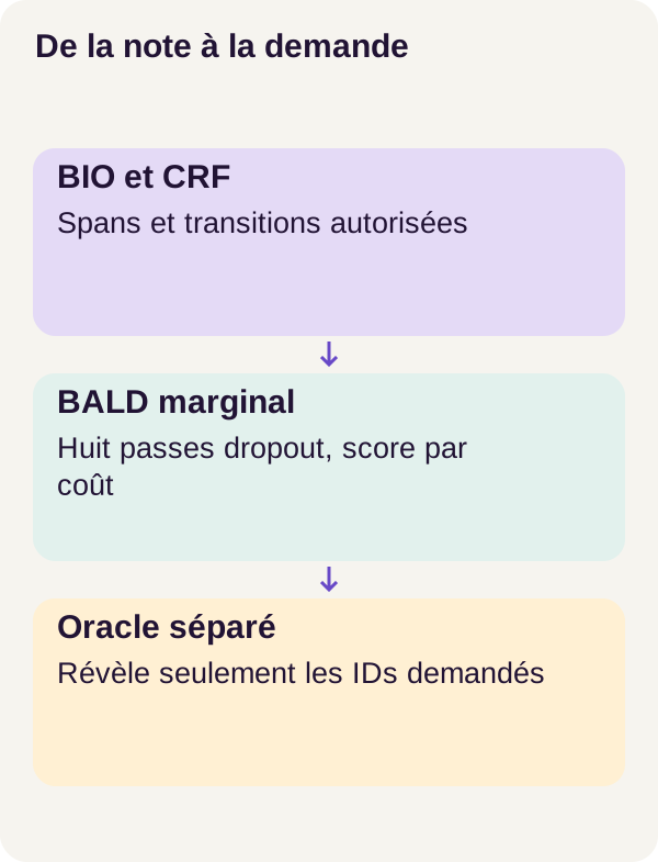
We will build this loop on fictional notes. A BiLSTM-CRF identifies entities in text, a selection queue chooses notes within a budget, then a separate oracle reveals only the requested annotations. We will explain these terms before running the project: this is neither asking a chatbot for answers nor developing a complete review interface.
The workflow is a reproducible demonstration, not a measurement of human productivity. The oracle is a program that already has the synthetic corpus’s correct answers. No annotator, delay, dropout or work time is observed. Cost is a published rule: 5 + number of tokens per note. We will retain this distinction when reading results.
Download the complete project, revision r001
Data and the no-leakage rule
Identifying an entity means recovering an exact text span
An entity here is a text portion assigned a type: REFERENCE, SITE or ECHEANCE. An annotation specifies both the type and the characters concerned. The model must learn to suggest the same information for a note whose annotations it does not know.
Consider this French sentence, included only to explain the mechanism (its original wording is retained so the character offsets remain valid):
Prévoir AX-14 à Lyon Nord avant le 18 octobre.
We want to identify AX-14 as a reference, Lyon Nord as a site and 18 octobre as a deadline. Such a portion is called a span. Offsets are its positions in the original text: they allow the correct occurrence to be highlighted, even if the same value appears multiple times.
In this teaching example, counting characters from zero and excluding the end boundary, AX-14 occupies [8, 13), Lyon Nord occupies [16, 25) and 18 octobre occupies [35, 45). The notation [8, 13) means ‘from character 8 inclusive to character 13 exclusive’. These are positions in this illustrative sentence, not a new project output.
The corpus preserves offsets, including accents, punctuation and hyphenated references. For a future interface, remember the issue: positions must always refer to the same text version. Changing spaces or characters after calculating offsets can shift highlighting.
Split notes before learning
The corpus contains 1,800 synthetic notes, organized into 120 families of 15 notes. It is split into 1,260 training notes, 270 validation notes and 270 test notes. Each note may contain a reference, site and deadline; their presence is not mandatory.
These three sets, often called splits, have different roles. Training supplies examples from which the model learns. Validation provides a separate set for development checks. Testing measures the result without feeding the pool’s annotation requests.
A family stays entirely within one set. This prevents variants from the same family being spread between training and testing. It does not make the corpus representative of a company: its vocabulary and grammar remain those of a controlled teaching generator.
Turn spans into BIO labels
The network does not directly receive strings to highlight. Text is divided into tokens, meaning units handled by the program, and each token receives a label. A token is not necessarily a whole word; the exact segmentation remains the project’s.
We use the BIO convention: B- marks an entity’s beginning, I- its continuation, and O a position outside the requested entities. With three types, we obtain seven labels: O, B-REFERENCE, I-REFERENCE, B-SITE, I-SITE, B-ECHEANCE and I-ECHEANCE.
To understand the convention, simply assume Lyon and Nord are successive tokens. We label Lyon with B-SITE, then Nord with I-SITE. The I- means ‘I continue an entity already started’, not ‘I start another category’.
Thus, I-SITE can follow only B-SITE or I-SITE. After O, the site must begin with B-SITE. After B-REFERENCE, we cannot continue directly with I-SITE: the type would change mid-entity.
The vocabulary is built from training texts only. Sentences form windows of at most 128 tokens, without overlap. Segmentation does not consult hidden annotations to choose a convenient boundary: if an entity crosses a boundary, the corpus is considered invalid. This restriction belongs to the demonstrated workflow; it is not a general solution for documents of every length.
The oracle must intervene only after selection
The random seed is 17. Here it selects 60 initial training notes, leaving 1,200 notes in the pool. The pool is the reserve of notes whose text is available but whose annotations have not yet been revealed to the learning workflow.
For a web developer, imagine two services with different permissions. The first can draw up a list of identifiers to process. The second holds annotations and returns them only for an authorized request.
The project makes this separation concrete: the process ranking the pool mounts neither the oracle nor hidden label files. It writes an ID request and computes a hash to identify the recorded request. The oracle then opens only requested files, rejects duplicates, notes outside training or inconsistent costs, and returns spans.
The hash identifies the request; lack of label access prevents reading labels during selection. These are different roles. A simple convention of ‘do not look at the answers’ would be less verifiable than a process that does not possess the files.
Without this separation, notes could be selected with prior knowledge of the model’s errors against their true annotations. We would no longer measure a strategy discovering answers progressively, but one assisted by the very answers it is supposed to request.
BiLSTM-CRF: from tokens to a valid sequence
The name combines two mechanisms. The BiLSTM provides context for each token. The CRF evaluates label sequences to produce one respecting BIO rules. Let us break down the path instead of treating the whole thing as a black box.
From identifiers to label scores
An embedding is a vector, or list of numbers, associated with a vocabulary token. Here, each vector contains 64 values, learned from scratch with the rest of the model. These representations are not retrieved from a large pretrained model. The torch.nn.Embedding documentation describes this lookup table between identifiers and vectors.
An LSTM, short for Long Short-Term Memory, is a network that traverses a sequence while retaining a state. The bidirectional version traverses it both ways. A token thus benefits from preceding and following context. With 64 units in each direction, the combined outputs give 128 values per token, consistent with the operation described in the LSTM 2.8 documentation.
Two dropout layers at 0.25 surround the LSTM. Dropout temporarily zeros randomly selected numerical components; it does not remove words from the note or permanently delete parameters. Its role in our uncertainty measurement appears in the next section.
Finally, a projection transforms the 128 values into seven emission scores, one per BIO label. An emission indicates how strongly the model favors a label at that position. This raw score is not yet a probability or a complete span.
For an illustrative ten-token window, the path is therefore: ten identifiers, then a 10 × 64 array, a contextualized 10 × 128 array and finally 10 × 7 scores. A tensor is simply the numerical array holding these values.
Why not choose the best label at every position?
Because a series of good local choices can form a forbidden sequence. Here is a small teaching calculation on Lyon Nord, reduced to three labels for readability. These scores are invented for explanation, not taken from training.
| Token | O score |
B-SITE score |
I-SITE score |
|---|---|---|---|
| Lyon | 3 | 2 | 0 |
| Nord | 0 | 1 | 4 |
Choosing the largest number in each row gives O → I-SITE, totaling 3 + 4 = 7. But this sequence announces a continuation without having started a site.
For this calculation, suppose all start, end and permitted transition scores are zero. The best legal sequence becomes B-SITE → I-SITE, scoring 2 + 4 = 6. The global choice is therefore not necessarily a succession of local maxima.
The CRF, or Conditional Random Field, assigns a score to an entire path. It combines emissions, a start score, an end score and transitions between successive labels. In this project, a transition is indexed in the previous-to-current direction.
Encode BIO rules in the calculation
The following code builds start and transition permissions. TAGS is the project’s label list; this excerpt runs in its environment, supplied in the ZIP.
def bio_constraints(tags=TAGS):
    start = torch.tensor([not t.startswith("I-") for t in tags])
    transitions = torch.ones((len(tags), len(tags)), dtype=torch.bool)
    for previous, a in enumerate(tags):
        for current, b in enumerate(tags):
            if b.startswith("I-"):
                transitions[previous, current] = a in ["B-" + b[2:], "I-" + b[2:]]
    return start, transitions
start is a boolean array: a true value permits a label to start the sequence. The three I- labels are therefore forbidden at the start.
transitions is a 7 × 7 matrix, initially filled with true values. The loop examines each pair. If current label b starts with I-, b[2:] retrieves its type, for example SITE. The transition remains permitted only if the previous label is B-SITE or I-SITE.
By contrast, a B- can start a new entity and O can leave an entity. The function defines what is permitted, not the learned score of each transition. The CRF then uses these constraints during training and decoding.
This distinction matters: the project does not produce an illegal sequence and repair it afterward. Forbidden paths are excluded from the intended calculation. A valid sequence can nevertheless be wrong: nothing prevents a model from selecting the wrong site while perfectly respecting BIO.
Learn with all paths, predict with the best
Two calculations use the same set of permitted paths but answer different questions.
Viterbi finds the best path. It retains the best intermediate scores and corresponding predecessors, then traces those choices backward at the end. This backtracking reconstructs the full sequence. It avoids explicitly enumerating every label combination.
Normalization logZ sums the weight of every permitted path. Each score becomes a positive weight through exponentiation. Z is their sum and logZ its logarithm. A path’s probability is then exp(path_score - logZ).
The loss function, called NLL for negative log-likelihood, is logZ - score_gold. Here, gold denotes the reference sequence revealed for training. Reducing this loss pushes the model to assign greater probability to the correct sequence relative to other legal paths. The PyTorch BiLSTM-CRF tutorial develops the distinction between normalization and decoding.
In our two-token example, the five legal paths have scores 3, 4, 2, 3 and 6. We obtain logZ ≈ 6.2257. If the reference is B-SITE → I-SITE, its loss is approximately 0.2257 and its probability approximately 0.7979. Being the best path does not mean having probability 1.
The calculation operates in log-space to limit numerical difficulties. The log-sum-exp operation stably calculates the logarithm of a sum of exponentials. It does not replace the sum with the maximum: that would change the problem.
Obtain a probability per token without forgetting context
To select notes for annotation, we need CRF marginals: the probability of each label at each position, accounting for complete paths. ‘Marginal’ means aggregating possibilities concerning other positions to focus on this one.
This is not a simple softmax independently applied to the seven emissions. The forward-backward calculation combines contributions arriving at a position and leaving it. Under the project’s convention, the formula is exp(alpha + beta - logZ). At each real token, the seven probabilities must sum to 1.
In this workflow, the calculation uses FP64 precision from FP32 emissions to limit rounding errors. GPU training remains FP32: the entire network is not switched to double precision. The small lattice used to explain paths has three tags; the tutorial model does use seven.
Uncertainty: what BALD actually approximates
We now know how to predict entities. We still need to select the next notes to annotate without looking at their answers. The strategy studied compares multiple predictions from the same network with dropout active.
Vary the calculation without training eight models
The workflow performs eight passes with dropout. Learned parameters remain the same, but dropout masks vary and produce eight marginal distributions per token. This repetition is called Monte Carlo dropout: multiple random calculations approximate a quantity not calculated exactly.
Standard PyTorch dropout is active during training and disabled in evaluation mode. To estimate disagreement, this variation must therefore be retained during the passes intended for that purpose. This is neither eight new training runs nor eight independent annotation teams.
BALD denotes a disagreement-based active learning criterion. In its Bayesian framework, it targets the information an answer could provide about model parameters. The paper on BALD with dropout presents an approximation using stochastic passes. Here, we apply this type of calculation to a CRF’s token marginals, not directly to all its possible sequences.
Being uncertain in the same way is not disagreement
Entropy measures how spread a distribution is across possibilities. With two choices of probabilities 0.5 and 0.5, it is higher than with 0.9 and 0.1. The project uses the natural logarithm; entropy values are therefore not percentages.
For a token, we calculate the entropy of the mean distribution minus the mean entropy. The first considers predictions together; the second considers how uncertain each pass is individually.
Take two passes and two labels solely to calculate by hand. The project uses eight passes and seven labels, but the subtraction is the same.
First case: both passes answer [0.5 ; 0.5]. Their mean is [0.5 ; 0.5]. The entropy of the mean is approximately 0.6931, as is the mean entropy. Calculated disagreement is therefore 0. The passes are uncertain, but identically so.
Second case: one pass answers [0.9 ; 0.1], the other [0.1 ; 0.9]. The mean remains [0.5 ; 0.5], so its entropy stays 0.6931. Each pass is more decisive, however: its entropy is approximately 0.3251. The difference reaches approximately 0.3681.
The mean distribution is identical in both cases, but disagreement is not. This is what the subtraction distinguishes. Conversely, multiple passes may be highly certain of the same wrong answer: a low score does not guarantee a correct annotation.
From token disagreement to note priority
The program sums real-token contributions across a note’s windows, then divides by its cost: 5 + number of tokens. Padding, added to group sequences of different lengths, is excluded by a mask. Padding facilitates batch computation; it must not create fictional information.
The score is therefore a cost-normalized, token-wise marginal approximation of the BALD type. Tokens are linked by the CRF; summing contributions does not compute the entire sequence’s exact conditional mutual information and may count dependent signals. The result is neither an error probability nor a measure of annotation’s human benefit.
Here is the source function. probabilities has shape M × T × K: number of passes, positions and labels. In the workflow, M = 8 and K = 7.
import math
import torch


def marginal_bald_score(probabilities, mask, cost):
    # M x T x K; sum token-wise proxy, not joint-sequence mutual information.
    if (
        probabilities.ndim != 3
        or probabilities.shape[1] != len(mask)
        or probabilities.shape[0] < 2
        or cost <= 0
        or not torch.isfinite(probabilities).all()
        or (probabilities < 0).any()
    ):
        raise ValueError("Invalid dropout marginals/cost")
    if not torch.allclose(
        probabilities[:, mask].sum(-1),
        torch.ones_like(probabilities[:, mask, 0]),
        atol=1e-5,
    ):
        raise ValueError("Real-token marginals must normalize")
    entropy = lambda p: -(
        torch.where(p > 0, p * torch.log(p.clamp_min(1e-30)), torch.zeros_like(p))
    ).sum(-1)
    values = entropy(probabilities.mean(0)) - entropy(probabilities).mean(0)
    if values[mask].min() < -1e-5:
        raise ValueError("Negative information proxy beyond rounding tolerance")
    return float(values[mask].clamp_min(0).sum() / cost), values.masked_fill(~mask, 0)
The first block checks, among other things, the three dimensions, agreement between position count and mask length, at least two passes, non-finite or negative values and a cost at or below zero. The next block checks that each real-token distribution sums to 1. An array of positive numbers alone does not constitute coherent probabilities.
The small entropy function sums over the last dimension, the labels. Zero handling prevents them contributing a log(0); clamp_min(1e-30) protects the logarithm’s argument. Then probabilities.mean(0) averages passes before calculating entropy, while entropy(probabilities).mean(0) averages already calculated entropies.
In exact arithmetic, this difference is nonnegative for valid distributions. The -1e-5 threshold tolerates tiny rounding differences; a more negative value raises an error. clamp_min(0) removes those small negative residuals from the summed score.
The function returns two objects: a scalar score divided by cost and a contribution vector whose padding positions are zeroed. This second object retains values before the score’s clamp_min(0); very small negative residuals can therefore still appear there.
The excerpt assumes a boolean mask containing at least one real token and a finite scalar cost. It does not itself check every prerequisite or recalculate cost from text. Cost consistency checking by the protocol and oracle remains a separate stage. Silently changing a distribution or cost to avoid rejection would change the experiment.
Spend a budget, not fill a document quota
Under our rule, a twenty-token note costs 25 units. That is not twenty-five seconds. The 5 represents a fixed simulated-cost component, and token count its variable component.
Another teaching example: a note with total contributions of 0.6 and cost 100 receives priority 0.006. Another, totaling 0.4 with cost 40, receives 0.01. The second comes first despite its lower raw contribution, because ranking is per unit of cost.
The baseline is random selection with deterministic priority and without replacement: once selected, a note does not return to the annotation pool. ‘Deterministic’ here means the same workflow can recover the intended order, not that the order exploits model uncertainty.
Random selection and BALD share the initial 60 notes, caps, architecture and test. Each cycle adds at most 4,000 units. A note that does not fit the remaining budget is skipped, then the queue continues. With 30 units left, a note costing 35 can be skipped while a later one costing 20 still fits: this example illustrates the rule without adding a workflow measurement.
We obtain ranking with budget control, not proof that the selected set is optimal. Two strategies can finish the same number of cycles with different expenditures. We will therefore compare F1 against actual cumulative cost consumed, not just cycle number.
Run the 21 verified commands
Prepare the environment and verify calculations
You should be able to read Python and use a terminal with Docker. Useful concepts include tensors, probabilities, sequences and gradients. The preceding examples provide reading guidance; code blocks belong in the complete project, not an isolated script to reconstruct.
The reference profile uses Linux and a 24 GiB RTX 3090, with 16 GiB of RAM and 10 GiB of working disk space, plus Docker storage. These are preparation recommendations, not measured minimums across all configurations. RAM is machine memory; the card’s 24 GiB is video memory.
Docker-to-NVIDIA-GPU integration must work. The NVIDIA Container Toolkit documentation describes this integration. A GPU visible on the host is insufficient: check_environment.py performs a BiLSTM-CRF forward and backward inside the container. Forward computes scores from inputs; backward calculates gradients needed for learning.
Extract the ZIP into a new directory and open a terminal at its root. All following commands run from this folder. We will execute the 15 main-workflow commands, the exercise command and five final commands, totaling the 21 commands in the supplied workflow.
sh scripts/preflight.sh
sh scripts/setup.sh
docker compose config --quiet
docker compose build acquisition tutorial learning inference initialization oracle
docker compose run --rm --no-deps acquisition python scripts/acquire.py --config configs/minimum.yaml
docker compose run --rm --no-deps tutorial python scripts/check_environment.py
docker compose run --rm --no-deps tutorial python -m pytest -q
Preflight checks the environment; setup prepares the project; Compose validates configuration and builds services. Acquisition checks an empty registry: no pretrained model is required. This stage therefore need not download an LLM or external embeddings.
The environment check then verifies computation inside Docker, and pytest runs project tests. A zero exit code indicates each command’s success. Program tests do not replace entity-quality measurement, which comes later.
Create the corpus and reveal the first annotations
Services have different roles. initialization launches bootstrapping operations; oracle reveals permitted annotations; training and inference roles remain separate. Compose mounts implement the intended access. Computations are isolated from the network and the oracle reserves no GPU.
docker compose run --rm --no-deps tutorial python -m ged_annotation_active_entites.cli prepare --config configs/minimum.yaml
docker compose run --rm --no-deps initialization python -m ged_annotation_active_entites.cli request-initial --config configs/minimum.yaml
docker compose run --rm --no-deps oracle python -m ged_annotation_active_entites.cli reveal --config configs/minimum.yaml
docker compose run --rm --no-deps initialization python -m ged_annotation_active_entites.cli baseline --config configs/minimum.yaml
docker compose run --rm --no-deps initialization python -m ged_annotation_active_entites.cli predict --config configs/minimum.yaml --cycle 0
prepare builds the corpus and its splits. Check counts 1,260 / 270 / 270 and family separation before interpreting a metric.
request-initial requests the initial 60 notes, then reveal provides their spans. The operations remain separate: the request exists before annotations are returned. The baseline command builds the starting point and predict --cycle 0 produces predictions for this initial cycle.
Cycle 0 is not the untrained model. It is the comparison point obtained after learning from initial annotations, before four additional annotation cycles. Confusing these states would completely change the result’s interpretation.
Inspect the mechanism before adding cycles
docker compose run --rm --no-deps tutorial python -m ged_annotation_active_entites.cli inspect-mechanism --config configs/minimum.yaml
This stage connects calculations to their representations. For a sequence, distinguish the selected BIO path from marginal distributions. Check that each real token has a distribution with total mass 1 and that padding positions do not contribute to the selection score.
The simplified three-tag lattice helps explain the mechanism; it does not describe reducing the actual model to three labels. Likewise, the article’s small numerical examples are explanations, not new training results.
Run four cycles, then evaluate
sh scripts/run_all.sh
docker compose run --rm --no-deps tutorial python -m ged_annotation_active_entites.cli evaluate --config configs/minimum.yaml
run_all.sh chains selection, revelation and training across four cycles. Acquired annotations progressively enrich the training set. Each strategy respects its caps but does not necessarily request the same notes.
At each cycle, the model restarts from the same untrained parameters, then learns for eight epochs on the annotations currently available. An epoch is one pass through training examples; an annotation cycle includes selecting new notes and the subsequent training. Eight epochs therefore do not mean eight new annotation requests.
This is not continuous fine-tuning of the previous cycle’s model. Annotations accumulate, but weights restart from the same initial state each cycle. This fixes comparison conditions for strategies; reusing previous-cycle weights would constitute a different experiment.
The optimizer is AdamW, with lr=0.003, weight_decay=0.001, a batch size of 16 and clipping at 1. A batch is a group of examples processed during training. Gradients describe how loss varies with parameters; the optimizer uses them to make adjustments. The lr rate controls update magnitude, while weight decay regularizes weights. The AdamW documentation details this mechanism.
Clipping limits gradient magnitude under the project’s rule. It limits neither F1 nor the number of selected notes. For the principle of norm limiting, the clip_grad_norm_ documentation provides further explanation.
Resuming an interruption is not restarting a cycle
The workflow also checks an interruption after epoch 4 of cycle 2. This time, training already in progress must resume, not return to the cycle’s initial parameters.
The checkpoint must restore the model, optimizer, sampler organizing sampling, RNGs or pseudo-random generators, pool, request and annotations. Restoring weights alone is insufficient: a different queue or new dropout draws can change what follows.
The check requires future selections and predictions to remain identical to those of the uninterrupted workflow. This is stricter than obtaining the same final F1: two models can have the same score without following the same experiment.
This verification concerns the reproduced environment. The PyTorch reproducibility documentation notes that an identical seed does not guarantee identical results after a version or platform change.
Read F1 and cost through an example
An almost correct boundary remains an extraction error
The measurement concerns exact spans: character boundaries and type must match the reference. It does not merely check whether some words overlap.
If the reference expects AX-14 but the model predicts only AX, the exact expected entity is missing: this is a false negative. It has also emitted an entity that does not match the reference: a false positive. The two counts do not represent two erroneous notes; they describe both sides of one incorrect extraction.
Precision measures the proportion of predicted spans that are correct. Recall measures the proportion of expected spans retrieved. F1 combines both with a harmonic mean so that good precision does not hide poor recall, or vice versa.
Return to the workflow’s example: 8 correct spans, 2 extra predictions and 2 missed spans. Precision is 8 / (8 + 2) = 0.8, recall is also 0.8, and F1 is 2 × precision × recall / (precision + recall) = 0.8.
The report retains entity types, their supports, meaning reference counts, and boundary diagnostics. These details help explain an error; they do not turn a partial match into success for exact F1.
Put budget, not cycle, on the horizontal axis
The curve places F1 on the vertical axis and annotation units actually consumed on the horizontal axis. Cycle number is insufficient: two queues may request notes of different lengths and spend different costs.
For example, comparing one method after 3,000 units with another after 4,000 does not directly measure quality at equal budget. Corresponding points would be needed. The workflow does not manufacture a gain by interpolating between different budgets.
Finally, only one seed is run. There is neither a three-seed average nor an uncertainty band around the curves. Reproducing a workflow exactly checks reproducibility; it does not measure variability from other initial draws.
Main workflow results
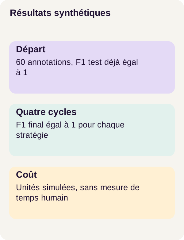
On the 270 test documents, exact F1 is already 1 after the initial 60 annotations. It remains 1 after four additional cycles for both main strategies: random selection and BALD.
Published final costs are 18,661 units for random selection and 18,620 for BALD. The 41-unit difference comes from selection order and note costs. It does not correspond to saved work minutes.
What can we conclude? The model already succeeds on the test at the comparison’s starting point. Adding annotations cannot increase F1 when it is already 1. The corpus and starting point therefore no longer distinguish strategies by this measure.
This result demonstrates neither a BALD gain nor its general uselessness. Nor does it prove that 60 annotations are the minimum required: we have not measured every smaller budget. Success concerns these synthetic notes and this test, not documents in a real EDM system.
The loop nevertheless retains educational value: authorized requests, controlled cost, distinct selections, training and resumption are observable. We learn to verify the mechanism without turning a ceiling score into a demonstration of profitability.
Hypothesis, then a redundancy exercise
Predict before running the scenario
Imagine the top notes ranked by BALD/cost have many closely related paraphrases. The model may give them high scores without each adding as much novelty as a genuinely different note.
Before running the exercise, write your hypothesis: will two near-copies of each of the ten initially top-ranked notes concentrate selection on repeated information? Can a diversity filter prevent this, and what might it discard along the way? Separate your cost prediction from your F1 prediction: they need not move together.
The supplied filter uses Jaccard similarity with a threshold of 0.85. To understand the formula, take two sets of elements: their similarity is the number of shared elements divided by the number present in at least one set. Identity gives 1; no shared elements gives 0.
In a mathematical example, 9 shared elements in a union of 10 give 0.9, above 0.85. Eight shared elements in a union of ten give 0.8, below it. These small sets illustrate the threshold; they do not replace the exercise code’s representation and comparison rule. The SciPy Jaccard documentation describes its distance version, equal to 1 - similarity: do not confuse the scores’ directions.
High similarity is not necessarily unhelpful redundancy. Two sentences can be almost identical while an important reference or deadline changes. The filter limits one form of closeness; it does not inherently know which annotations will be most useful.
Run, then compare with your hypothesis
sh scripts/run_exercise.sh
The scenario creates two near-copies per affected note, then reruns four cycles for BALD alone and four for BALD with filtering. The test, vocabulary and initial 60 annotations stay fixed. No F1 gain or savings are imposed on the experiment.
The answer is to compare cost, covered types and F1, without changing the test after observing results. Covered types notably help check that selection does not concentrate all its attention on a single entity category.
In the supplied result, final F1 remains 1 in both variants. Costs are 18,645 units with duplicates and 18,617 with the diversity filter, a difference of 28 units. These values belong to the exercise; they do not replace main-workflow costs.
The filter changes selection and simulated expenditure, but the ceiling measurement shows no quality improvement. We therefore cannot claim diversity is universally useful or convert this difference into saved annotation time.
Generate figures and clean up
After comparing the exercise with your hypothesis, generate figures and check checkpoints. Retain useful outputs after the first two commands and before cleanup, because clean.py --outputs-only will erase results.
docker compose run --rm --no-deps tutorial python lesson/figures/plot.py
docker compose run --rm --no-deps tutorial python scripts/check_checkpoints.py
docker compose down
docker compose run --rm --no-deps tutorial python scripts/clean.py --outputs-only
docker compose down
plot.py generates figures from outputs. check_checkpoints.py checks saved files. The docker compose down commands then surround project cleanup.
The cleanup script displays and deletes only outputs. It removes neither the corpus nor checkpoints nor other Docker projects’ files. This is also why a divergent checkpoint should be retained for inspection instead of deleted before understanding the discrepancy.
Troubleshooting, cleanup and product limits
Find the cause of a discrepancy
Docker cannot see the GPU. Follow the preflight diagnosis and retry in a newly extracted folder. Distinguish card visibility in Linux from successful computation in the container; check_environment.py checks that second stage.
A marginal distribution is rejected. Examine dimensions, non-finite or negative values, normalization over real tokens and the mask. A positive cost also does not establish that it matches the requested note: the oracle checks that consistency separately. Do not replace probabilities with arbitrary numbers to obtain a score.
An annotation crosses a window. The corpus no longer respects the workflow’s segmentation contract. Moving the boundary by consulting hidden labels would bypass precisely the rule being studied. For a new corpus, an appropriate segmentation strategy must be defined and evaluated rather than hiding the error.
Resumption diverges. Keep checkpoints and inspect the model, optimizer, sampling order, random states and annotation queue. Different final outputs can come from incompletely restored state, not only a bad model. Targeted cleanup remains as described in the preceding section.
What a real annotation team still needs
The tutorial replaces humans with a perfect oracle. A real application must instead define entities with domain teams, train annotators and measure their time, costs, errors and abandonment. An ambiguous reference, imprecise deadline or disagreement between people cannot be reduced to token count.
The team must have the necessary consent and access rights for documents it uses. It must retain text, offsets and revisions, plan for new entity types and handle errors from the real oracle—whether a person or a validation process.
The product layer also requires authentication, APIs, logs, monitoring, load tests, backup, restoration and human review. These are tasks to plan, not features already demonstrated by this learning loop.
Finally, the model suggests spans to correct; it validates no status, person or access. Detecting a date in a note does not certify that the deadline was approved. The interface’s role would be to present a suggestion and its source without confusing them with a business decision.
Summary
We started with a practical question: which notes should be annotated next? The BiLSTM turns tokens into contextualized scores; the CRF organizes those scores into permitted BIO paths and provides marginals. Dropout passes then construct a disagreement score normalized by an explicit cost.
Selection makes sense only if it does not already know the answers. Separating hidden labels, requests and the oracle makes this condition verifiable. Budget control and state resumption allow exact tracking of what was requested and learned.
Three distinctions remain essential: BIO validity versus span correctness; model disagreement versus error probability; simulated cost versus human work. One measurement cannot substitute for another.
On this corpus, every presented strategy reaches F1 = 1. The absence of an observed gain is the result to retain, not a defect to hide. The workflow teaches us to build and examine an active annotation loop; it does not demonstrate improved team productivity.
Primary sources and further reading
The data, parameters, commands and results presented belong to the r001 project linked at the start. Sentences, small lattices and calculations added for explanation are teaching examples separate from workflow measurements.
The main references are the PyTorch BiLSTM-CRF tutorial, the torch.nn.LSTM 2.8 documentation and the BALD with dropout paper. Supplementary links throughout the text detail embeddings, dropout, numerical calculations, optimization, reproducibility, Jaccard and GPU access.
This documentation explains the mechanisms; it does not replace the ZIP’s files and dependencies for reproducing revision r001.