





You may already have optimized a web process that looped through the same array several times. The idea seemed simple: combine the operations to avoid intermediate work. But before comparing timings, you had to check that the new version still produced the same result.
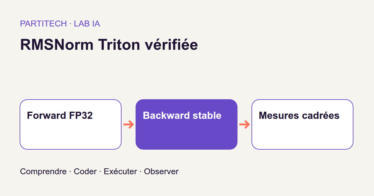
We will follow that approach inside a neural network. Our operation is called RMSNorm: it rescales lists of numbers. We will start with a readable PyTorch version, then combine its computation into a Triton kernel, a function executed on the GPU. An additional challenge awaits us: during training, getting the right output is not enough. We also need to compute the right gradients.
The walkthrough produces an RMSNorm connected to Autograd, used in a small network that is actually trained and then reloaded. Its aim is to verify the computation within a specific scope, not to demonstrate that “Triton is always faster.” We will examine numerical correctness and latency separately.
Problem and reference formula
What exactly are we normalizing?
A network transforms its inputs into sequences of intermediate numbers: these are its activations. They change from one example to another. Weights, meanwhile, are the parameters that training adjusts to change the network's behavior.
Here, normalizing activations means controlling their scale. We are not fixing a string or a document's format: we are applying a numerical transformation inside the model.
In this project, the input x is a two-dimensional array, called a tensor. A tensor can have more dimensions, but here we stick to a matrix with M rows and N columns. Each row is normalized independently of the others.
| Object | Shape in this tutorial | How to read it |
|---|---|---|
x |
M × N |
M rows of activations, with N numbers per row. |
gamma |
N |
One weight per column, shared across all rows. |
r |
One number per row | The inverse of the scale measure computed for that row. |
y |
M × N |
The activations obtained after normalization and multiplication by gamma. |
RMS stands for root mean square. Squaring prevents positive and negative values from canceling each other out. The mean accounts for the row's length; the square root brings us back to a measure of scale.
For one row, the reference formula is:
r = 1 / sqrt(mean(x²) + epsilon)
y = x × r × gamma
Multiplication is elementwise. r is shared by the entire row, but each column has its own gamma. The small number epsilon, set to 1e-6 in the functions shown, is added before the square root. In particular, it prevents division by zero for an all-zero row.
Let's work through two values
Take x = [3, 4], gamma = [1, 1] and epsilon = 1e-6. This is an arithmetic illustration, not a row taken from the GPU measurements.
| Step | Calculation | Approximate result |
|---|---|---|
| Squares | [3², 4²] |
[9, 16] |
| Mean of squares | (9 + 16) / 2 |
12.5 |
| Stabilized denominator | sqrt(12.5 + 0.000001) |
3.535534 |
Inverse r |
1 / 3.535534 |
0.282843 |
| Output | [3 × r, 4 × r] |
[0.848528 ; 1.131371] |
We have preserved the ratio between the two values while changing their scale. The second output exceeds 1: normalizing does not mean constraining every number to the range from 0 to 1.
Change only gamma to [2, 0.5]. The output becomes approximately [1.697056 ; 0.565685]. These weights let the network adjust the importance of each coordinate separately after rescaling. They are therefore not merely a cosmetic setting.
Unlike LayerNorm, RMSNorm does not subtract the row's mean. In our example, both outputs remain positive: their mean is not zero. The original RMSNorm paper presents this distinction; the PyTorch RMSNorm documentation also gives its formula. Our comparison, however, will use the reference written in this tutorial, with its explicit choices of precision and epsilon.
Why do we need a forward and a backward pass?
The forward pass computes y from x and gamma. During training, the network then produces a prediction, compared with a target through a loss: a number we seek to reduce.
The backward pass, or backpropagation, propagates gradients in the opposite direction. A gradient measures how sensitive the loss is to a small change in a value. It does not update weights itself: the optimizer uses it to do so.
At the input to RMSNorm's backward pass, dy means “gradient of the loss with respect to y.” It is neither the difference y - x nor directly the error between the prediction and the target. The operations after RMSNorm have already contributed to its calculation.
We need to return two objects: dx, to continue backpropagation toward the previous layer, and dgamma, to learn the normalization weights. With u = dy × gamma, the expressions we need to obtain are:
dx = r × u − x × r³ × mean(u × x)
dgamma = sum_rows(dy × x × r)
We will explain these formulas when we implement them. For now, note the difference: the mean in dx is over the N columns of one row, whereas the sum in dgamma is over the M rows.
PyTorch provides tensor operations and Autograd organizes their derivatives. Triton lets you write GPU computations with Python-like syntax. A kernel groups operations to run on the card; it is not a pretrained model. Here, we must explicitly provide its backward pass to connect it to the rest of the network.
Docker and GPU prerequisites
You should know how to read a Python function, work with arrays and use a terminal with Docker. No prior CUDA programming experience is needed to follow the explanations.
The validated walkthrough requires Linux x86_64, Docker with Compose, NVIDIA Container Toolkit and one 24 GiB RTX 3090. Allow 16 GiB of RAM and 16 GiB of disk space, excluding shared Docker layers. The GPU's video memory, or VRAM, is separate from system RAM. No CPU profile substitutes for the kernel's CUDA execution.
Extract the archive and open your terminal at its root. All the following commands run from this same directory. The article's snippets show the central functions, not standalone files: imports, the full contract and helper functions remain in the downloadable project.
setup.sh creates local directories and writes only UID/GID to .env: these identifiers are used to manage file permissions. Here, acquire downloads neither a pretrained model nor an external dataset. The data will be synthetic; outputs/ receives the checks and artifacts/ the checkpoints, meaning the network's saved states. Dependencies are resolved and checked during the build.
sh scripts/setup.sh
docker compose config --quiet
docker compose build acquire gpu
docker compose run --rm acquire python scripts/acquire.py --config configs/minimum.yaml
docker compose run --rm gpu python scripts/check_environment.py --config configs/minimum.yaml
docker compose config --quiet checks the Compose configuration. The build prepares the acquire and gpu services. Finally, check_environment.py initializes CUDA in the container and performs a computation: seeing a card from Linux is not enough to prove it is usable from Docker.
If that last check fails, stop at this step and check the integration using the NVIDIA Container Toolkit guide. Do not change the RMSNorm formula to work around an environment problem. Reusing Docker layers can change build time; it does not change the numerical computation we will compare.
Check the safeguards before the kernel
Before optimizing a web function, you would keep tests for its inputs and outputs. We do the same with GPU computation, adding checks for gradients and memory layout.
The public suite covers irregular sizes, the memory contract, negative cases and gradient checks. A negative case is an input that must be rejected, or an incorrect variant the test must detect. Correctly detecting an expected error therefore counts as a passing test.
docker compose run --rm gpu python -m pytest -q
The suite must finish without failures before measurements or training. That success applies to the project's code and cases: it does not turn our operator into a universal kernel accepting any size, numeric type or memory layout.
PyTorch reference: the numerical oracle
A test oracle is simply a version against which we compare the implementation under study. Our reference prioritizes readability: we can relate each Python line to the formula above.
A tensor's dtype is its numeric type. FP16, FP32 and FP64 refer to floating-point numbers stored in 16, 32 and 64 bits. Their precision differs. The reference works in float64 if the input is already float64, otherwise in FP32; it then converts the output back to the input's type.
def rmsnorm_reference(x, gamma, epsilon=1e-6):
    dtype = torch.float64 if x.dtype == torch.float64 else torch.float32
    xf = x.to(dtype)
    gf = gamma.to(dtype)
    r = torch.rsqrt(xf.square().mean(-1, keepdim=True) + epsilon)
    return (xf * r * gf).to(x.dtype)


def manual_backward(x, gamma, dy, epsilon=1e-6):
    r = torch.rsqrt(x.square().mean(-1, keepdim=True) + epsilon)
    u = dy * gamma
    dx = r * u - x * r.pow(3) * (u * x).mean(-1, keepdim=True)
    dgamma = (dy * x * r).sum(0)
    return dx, dgamma
Reading the forward pass line by line
xf and gf are working versions of x and gamma, converted to the chosen type. square() computes the squares. mean(-1, keepdim=True) computes the mean along the last axis, hence across columns.
Why retain the dimension with keepdim=True? For an M × N input, the mean has shape M × 1. Each row thus retains its own number, which PyTorch can multiply across all columns of that same row. This automatic shape expansion is called broadcasting. Meanwhile, gamma, with shape N, is reused across all rows.
torch.rsqrt(a) computes 1 / sqrt(a). The last line therefore applies exactly x × r × gamma, then restores the original dtype. Computing temporarily in FP32 does not mean the output will remain FP32 if the input was FP16.
An independent, readable backward formula
manual_backward() expresses both derivatives without using Triton. Its purpose is to compare an explicit formula with the gradients produced by Autograd.
Unlike rmsnorm_reference(), this function does not explicitly convert its inputs to a higher-precision type. It must therefore be read with its arguments' dtypes in mind; by itself, it is not a recipe for FP32 reduction on FP16 tensors. The kernel, by contrast, will make this conversion visible in its loads.
Gradcheck adds another verification: it slightly perturbs inputs and compares the numerical variation of the output with the computed derivative. To understand the idea, the slope of a scalar function can be estimated by (f(a + h) - f(a - h)) / (2 × h), with a small h. The gradcheck documentation explains, in particular, the role of double precision in its usual settings.
In this walkthrough, float64 gradcheck applies to the PyTorch reference, not the FP32/FP16 Triton kernel. The kernel will be compared in separate checks. This distinction prevents us from attributing to one program a test run on another.
Now generate this reference check and the three synthetic splits:
docker compose run --rm gpu python -m rmsnorm_kernel.cli reference --config configs/minimum.yaml
The splits separate data intended for training, validation and testing. Their generation details are in the project; no business data or external model is needed to study this operation.
Triton forward: one row, one program
The memory contract is part of the computation
Imagine a function that accepts a rectangular array but traverses its memory as if every row were stored consecutively. It would be incorrect on a view whose elements are spaced differently, even if the displayed dimensions looked right.
Here, a contiguous tensor has the compact layout expected by the kernel. Strides describe the steps in memory needed to move to another row or column. A transpose, for example, can produce a noncontiguous view without moving all the numbers.
Before writing to outputs, the project's contract rejects noncontiguous inputs, dtypes other than FP32/FP16, mismatched devices, an invalid epsilon, N greater than 4096 and temporary space, or scratch space, exceeding 64 MiB. The body of check_contract() is not reproduced below: retain the checks from the complete file.
@triton.jit
def rmsnorm_forward_kernel(
    X, G, Y, R, N: tl.constexpr, EPS: tl.constexpr, BLOCK: tl.constexpr
):
    row = tl.program_id(0)
    column = tl.arange(0, BLOCK)
    x = tl.load(X + row * N + column, column < N, other=0).to(tl.float32)
    gamma = tl.load(G + column, column < N, other=0).to(tl.float32)
    inverse = tl.rsqrt(tl.sum(x * x, 0) / N + EPS)
    y = x * inverse * gamma
    tl.store(Y + row * N + column, y, column < N)
    tl.store(R + row, inverse)


def forward_op(x, gamma, epsilon=1e-6):
    check_contract(x, gamma, epsilon)
    m, n = x.shape
    y = torch.empty_like(x)
    inverse = torch.empty(m, device=x.device, dtype=torch.float32)
    rmsnorm_forward_kernel[(m,)](
        x, gamma, y, inverse, n, epsilon, triton.next_power_of_2(n)
    )
    return y, inverse
Who computes which row?
The Python function forward_op() checks inputs, allocates outputs, then launches the kernel with the [(m,)] grid. This requests M instances of the Triton program, one per row.
tl.program_id(0) gives each instance its row number. This number represents neither a Docker process nor an additional graphics card. tl.arange(0, BLOCK) builds the column positions processed together. The first Triton tutorial introduces this programming model and its memory masks.
X + row * N + column addresses the values of the desired row. The formula uses N because actual rows contain N values. It does not use the rounded BLOCK size to move to the next row.
The @triton.jit decorator delegates kernel compilation to Triton. Parameters marked tl.constexpr are known during specialization: they describe, among other things, the block dimensions and constants for this computation, not learned weights.
N and BLOCK: two sizes you must never confuse
triton.next_power_of_2(n) chooses a working width equal to the next power of two. With N=257, the program therefore handles BLOCK=512 positions, but only columns 0 through 256 belong to the row.
This does not turn our tensor into a matrix with 512 columns. The extra positions are computation slots that need masking. tl.load(..., column < N, other=0) does not read values beyond the row: it substitutes zero for them. tl.store(..., column < N) writes only valid values.
Why zero? It does not change the sum of squares. However, it must not count as an extra observation in the mean. The sum must be divided by N, not by BLOCK.
Take a smaller example, separate from the measurements: a row [1, 1, 1] processed with a four-position block. The sum of squares of [1, 1, 1, 0] is still 3. Dividing by 3 gives the correct mean, 1; dividing by 4 gives 0.75. The mask protects memory accesses, but does not choose the right denominator for us.
The same flaw is invisible at N=256, because BLOCK is then also 256. That is why an irregular size is a useful test, not a presentation detail.
Why convert before reducing?
A reduction transforms several values into one result, such as a sum or mean. Here, numbers are converted to FP32 as soon as they are loaded, before squaring and summing them. Converting only after an already rounded computation would not recover the lost precision.
The kernel computes the inverse RMS, applies gamma, then writes y. Y has the same type as x, thanks to torch.empty_like(x); R stores one inverse per row, explicitly in FP32, for the backward pass. empty_like allocates memory without filling it with zeros: the kernel really must write every required output.
We have fused the forward pass, but have not eliminated all intermediate storage: R is deliberately retained between the forward and backward passes.
docker compose run --rm gpu python -m rmsnorm_kernel.cli check-forward --config configs/minimum.yaml
This check compares the forward pass at the planned sizes, including N values that are not powers of two. The Triton LayerNorm lesson explores normalization and reduction kernels in more depth; it does not replace this project's narrower RMSNorm contract.
Input backward pass: keep the right N
The challenge: every value also affects the denominator
To compute dx, we cannot simply multiply dy by r × gamma. That would ignore the fact that r itself depends on the entire row x.
Return to [3, 4]. If we change the first number, its numerator changes, but the sum of squares changes too. The denominator shared by both outputs therefore changes. The backward pass must account for this collective effect.
That is the role of the formula's two terms: r × u describes the direct effect; −x × r³ × mean(u × x) adds the effect of the change in normalization. u = dy × gamma first incorporates the per-column weights.
To illustrate this with the same example, reset gamma = [1, 1] and choose the illustrative upstream gradient dy = [1, 2]. We have u = [1, 2], then mean(u × x) = (3 + 8) / 2 = 5.5. With epsilon = 1e-6, the formula gives approximately:
dx = [-0.090510 ; 0.067882]
The first gradient is negative even though the values of dy are positive. This is not an anomaly: increasing an input can reduce other outputs by increasing their denominator. The gradient accounts for every path through which that input affects the loss. These numbers illustrate the formula; they are not the kernel's measured discrepancies.
Where does the cube of r come from?
This short derivation is optional for running the project, but makes the code less mysterious.
Let s = mean(x²) + epsilon. Since r = s^(-1/2), the derivative of r with respect to s is −(1/2) × s^(-3/2), or −r³ / 2. The derivative of s with respect to a coordinate x_i is 2 × x_i / N.
Multiplying the two gives ∂r/∂x_i = −x_i × r³ / N. We then need to sum the contributions of every output using that same r, which yields the second term of dx.
The cube is therefore not a setting to adjust until the test passes: it comes from differentiating the reciprocal square root.
@triton.jit
def rmsnorm_dx_kernel(X, G, DY, R, DX, PARTIAL, N: tl.constexpr, BLOCK: tl.constexpr):
    row = tl.program_id(0)
    column = tl.arange(0, BLOCK)
    x = tl.load(X + row * N + column, column < N, other=0).to(tl.float32)
    gamma = tl.load(G + column, column < N, other=0).to(tl.float32)
    dy = tl.load(DY + row * N + column, column < N, other=0).to(tl.float32)
    inverse = tl.load(R + row)
    u = dy * gamma
    mean_ux = tl.sum(u * x, 0) / N
    dx = inverse * u - x * inverse * inverse * inverse * mean_ux
    tl.store(DX + row * N + column, dx, column < N)
    tl.store(PARTIAL + row * N + column, dy * x * inverse, column < N)


def backward_rows(x, gamma, dy, inverse, epsilon):
    check_contract(x, gamma, epsilon)
    if (
        dy.shape != x.shape
        or dy.dtype != x.dtype
        or dy.device != x.device
        or not dy.is_contiguous()
    ):
        raise ValueError("dy must match x and be contiguous")
    m, n = x.shape
    dx = torch.empty_like(x)
    partial = torch.empty((m, n), device=x.device, dtype=torch.float32)
    rmsnorm_dx_kernel[(m,)](
        x, gamma, dy, inverse, dx, partial, n, triton.next_power_of_2(n)
    )
    return dx, partial
What this kernel produces
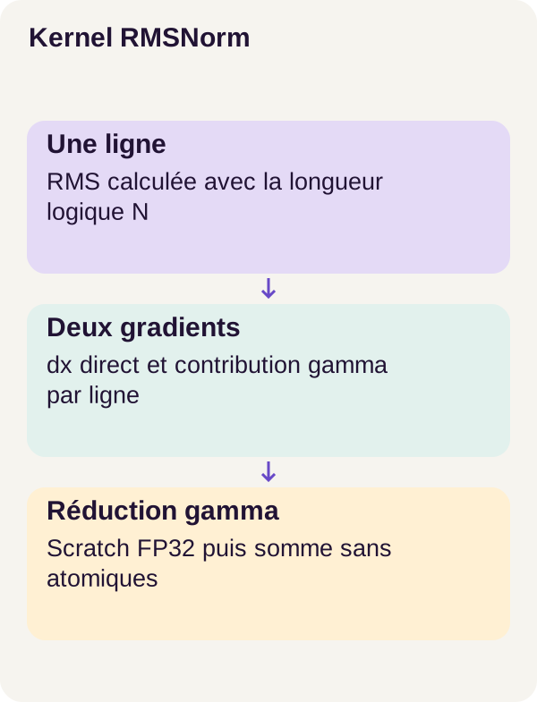
The program loads x, gamma, and dy in FP32, then retrieves the inverse saved during the forward pass. mean_ux adds u × x and, again, divides by N. Masked columns do not contribute to this sum.
It then writes two objects. DX receives the input gradient, in an output with the same shape and type as x. PARTIAL receives one contribution to dgamma for each row and column: dy × x × inverse. This array is not yet the final gradient for gamma; it will be reduced in the next step.
In backward_rows(), the additional check requires dy to have the same shape, dtype, and device as x, and to be contiguous. The future Autograd wrapper will call dy.contiguous() to meet that last condition. This does not make non-contiguous user inputs x and gamma acceptable: the contract still rejects them.
Here, the inverse is an internal intermediate, produced by forward_op() and retained for this calculation. This excerpt must not be interpreted as a public API that validates any inverse tensor supplied from outside.
Now check dx against the reference:
docker compose run --rm gpu python -m rmsnorm_kernel.cli check-backward --config configs/minimum.yaml
If the forward pass is correct but dx is not, inspect the derivative: a correct forward pass does not guarantee that we implemented its backward pass correctly.
Reducing dgamma without a write race
A shared weight receives several contributions
Each column uses the same gamma weight for every row. Its gradient must therefore collect the contributions from those rows. Picture several tasks, each calculating part of a total: we add their contributions rather than arbitrarily keeping the last one.
If all GPU programs tried to modify the same slot without coordination, we would have a write race. An atomic addition can prevent contributions from being lost, but the order of concurrent additions can vary. In floating-point arithmetic, that order can change the final digits of the result.
The teaching minimum uses another layout: each row writes to its own area of partial, then a second Triton pass adds those contributions by column. It reduces in FP32 before converting the result to the dtype of gamma. This choice avoids concurrent atomic accumulation here; it does not promise bit-for-bit identity across all hardware and versions.
def reduce_gamma_gradient(partial, dtype):
    m, n = partial.shape
    result = torch.empty(n, device=partial.device, dtype=dtype)
    gamma_sum_kernel[(triton.cdiv(n, 32),)](partial, result, m, n, 32, 32)
    return result
result has N elements, one gradient per weight. triton.cdiv(n, 32) is division rounded up: for N=257, it schedules nine programs. The body of gamma_sum_kernel is not reproduced in this excerpt; the full layout of this second reduction is available in the archive. The function above shows its launch and output type.
A sum is not an average
For a purely educational example, suppose two rows have already produced the following contributions:
| Contribution | Column 0 | Column 1 |
|---|---|---|
| Row 0 | 1 | 2 |
| Row 1 | 3 | 4 |
Expected sum for dgamma |
4 | 6 |
| Average, which would be incorrect here | 2 | 3 |
There is no additional division by M in the dgamma formula. If the overall loss already averages across examples, that weighting is passed through dy. Dividing again here would change the gradient of the operation.
With a single row, sum and average are identical. With 17 rows, they generally are not: that is why the M=1 and M=17 cases are useful for detecting a mix-up.
The cost of this layout: a temporary array
partial contains M × N FP32 numbers of four bytes each. Its footprint is therefore M × N × 4 bytes.
For the benchmark shape 128 × 257, this represents 131,584 bytes, or 128.5 KiB. This calculation concerns partial only, not all the program's VRAM. With M=4096 and N=4096, the same array reaches 64 MiB; one additional row exceeds that limit.
These calculations explain the scratch budget: an allowed width N is not enough to make every height M acceptable. They are not a new measurement of the project's memory.
docker compose run --rm gpu python -m rmsnorm_kernel.cli check-gamma --config configs/minimum.yaml
The check-gamma check completes the previous checks: it targets the shared-weight gradient, not only input gradients.
Connecting Autograd and actually training
We now have the forward pass, dx, and dgamma. They still need to be connected to PyTorch. That is the role of the torch.autograd.Function subclass.
For a web developer, it can be seen as an adapter: the rest of the program calls a regular operation, while the adapter knows how to delegate its execution and backward pass to specialised code. Autograd is not a tool that guesses our Triton formula: we explicitly provide the backward rule. The PyTorch documentation on custom functions describes this interface.
class RMSNormFunction(torch.autograd.Function):
    @staticmethod
    def forward(ctx, x, gamma, epsilon):
        y, inverse = forward_op(x, gamma, epsilon)
        ctx.save_for_backward(x, gamma, inverse)
        ctx.epsilon = epsilon
        CALLS["forward"] += 1
        return y

    @staticmethod
    def backward(ctx, dy):
        x, gamma, inverse = ctx.saved_tensors
        dx, partial = backward_rows(x, gamma, dy.contiguous(), inverse, ctx.epsilon)
        dgamma = reduce_gamma_gradient(partial, gamma.dtype)
        CALLS["backward"] += 1
        return dx, dgamma, None


def rmsnorm(x, gamma, epsilon=1e-6):
    return RMSNormFunction.apply(x, gamma, epsilon)
What ctx retains
ctx is the context of a function call. In the forward pass, save_for_backward(x, gamma, inverse) retains the tensors needed for the backward pass. epsilon, which is not a learned tensor in this contract, is retained separately as an attribute.
During the backward pass, we recover those same tensors. dy.contiguous() ensures a compact layout for the upstream gradient: this method returns the tensor when it already fits and makes a contiguous copy when needed, as stated in the documentation for contiguous().
backward_rows() calculates dx and intermediate contributions. reduce_gamma_gradient() adds them. Finally, return dx, dgamma, None answers the three input arguments, in the same order: one gradient for x, one for gamma, and none for epsilon.
This None does not mean epsilon has no mathematical effect on the output. It means that this parameter is not differentiated by our interface.
Gradients are not updates yet
No optimiser call appears in this class. It calculates outputs and returns gradients; the outer training loop then uses Adam to modify parameters. The CALLS counters record passes through the wrapper, not the exact number of GPU launches: one backward pass here calls the per-row calculation and then the gamma reduction.
The small network being compared is Linear → RMSNorm → SiLU → Linear. A Linear layer combines inputs with weights; SiLU adds a nonlinear transformation. Both paths start with identical initialisations, so we compare the reference and the kernel without giving them different starting points.
The walkthrough trains for 100 steps with Adam and 32 examples per step, reloads the weights, then checks that the kernel path called forward and backward 100 times. This check notably prevents us from validating training that mistakenly stayed on the reference path.
docker compose run --rm gpu python -m rmsnorm_kernel.cli train-integration --config configs/minimum.yaml
The integration check verifies that our operation actually takes part in learning. Reloading also verifies the saved weights. This is not the same claim as a complete resume after interruption with the whole optimiser state restored; that second scenario is not claimed here.
Measurements before results
Three distinct numerical comparisons
The checks cover 72 cases each for the forward pass, dx, and dgamma. We therefore compare outputs, input gradients, and weight gradients: three different objects.
The declared tolerances are atol=1e-5, rtol=1e-4 in FP32, and atol=rtol=3e-3 in FP16. Atol is an absolute margin; rtol adds a margin proportional to the reference value.
To read these parameters, the element-by-element closeness rule for torch.allclose is:
abs(value - reference) ≤ atol + rtol × abs(reference)
With the FP32 tolerances, a reference equal to 1 permits a difference of 0.00011. A reference equal to 100 permits 0.01001. These examples explain the calculation; they are not cases captured in the run.
A maximum absolute error alone is therefore not enough to conclude that a relative tolerance was exceeded. You need to know the dtype, the reference value, and the result of the relevant check. Conversely, a small mean error would not let us ignore one failing element.
Why not always require zero? Floating-point numbers have limited precision, and operation order can change rounding even for mathematically equivalent expressions. The PyTorch note on numerical accuracy describes this limit. We keep tolerances declared before the comparison rather than increasing them after seeing an error.
What time does the benchmark measure?
The protocol places CUDA events around complete calls. It retains allocations, the Autograd path, and related launches; it does not reduce the measurement to the Triton kernel body alone.
One clarification is useful: CUDA events measure an interval on the GPU timeline. They are not stopwatches that separately assign a CPU cost to each Python line. Their results therefore describe this execution scope, not a detailed breakdown of allocations, dispatch, and computation.
The warm-up runs operations before durations are recorded. Here, the 20 warm-up calls are excluded; medians are calculated from 50 samples of 20 calls. The two 20s do not have the same role: the first prepares the run, the second groups measured calls.
The median describes the middle of ordered observations, unlike the mean, which adds durations and divides by their number. It does not by itself describe the worst delays or full variability.
docker compose run --rm gpu python -m rmsnorm_kernel.cli benchmark --config configs/minimum.yaml
Walkthrough observations
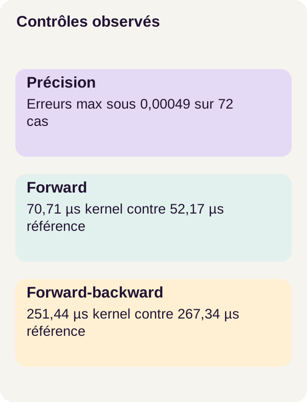
The following latencies are local measurements observed on an RTX 3090, for the 128 × 257 shape in FP32. The three error rows each summarise their 72-case run; this table does not break those maxima down by dtype. Do not assign them to an individual case that is not identified in the summary.
These figures do not predict the best kernel for another shape, another card, a comparison with torch.compile, or another timing scope.
On mobile, scroll the table horizontally.
| Observed check | Result |
|---|---|
| Maximum absolute forward error, 72 cases | 0.00024414 |
| Maximum absolute dx error, 72 cases | 0.00048828 |
| Maximum absolute dgamma error, 72 cases | 0.00012207 |
| Reference forward median | 52.17 µs |
| Kernel forward median | 70.71 µs |
| Reference forward + backward median | 267.34 µs |
| Kernel forward + backward median | 251.44 µs |
The integration gives an initial output error of 1.19e-7 and a gradient error of 5.96e-8. After 100 steps, the reference and kernel paths have a test MSE of about 0.30670 and reloading has a zero difference. MSE is the mean of squared differences between predictions and targets: it is not a success percentage. The kernel path did execute 100 forwards and 100 backwards.
These checks concern the small network and its synthetic data. They do not measure an improvement in a language model's understanding or in business quality.
The forward pass and training walkthrough do not tell the same story
The following table contains only differences calculated from the medians published above, not new measurements. The percentage divides the duration difference by the reference median.
| Scope | Kernel − reference difference | Duration change |
|---|---|---|
| Forward only | 70.71 − 52.17 = +18.54 µs |
About +35.54% |
| Forward + backward | 251.44 − 267.34 = −15.90 µs |
About −5.95% |
The isolated forward pass is therefore slower for this measured shape. The forward-backward pair is faster within this scope. A result can be numerically correct without improving latency for every use.
We do not infer a “pure backward time” by subtracting two medians from separate walkthroughs. Nor do we attribute the difference to a specific cause without further profiling. The provided figures do not detail that attribution or the full distribution of times.
For an application that only makes predictions, the forward pass matters directly. For a learning loop, the forward and backward passes both matter, but they still do not alone represent the complete network, optimiser, and data loading. The conclusion must stay tied to the work that was actually timed.
What we learned
We started with a mean of squares and built a complete path: a readable reference, a Triton forward pass, an input backward pass, a reduction for the shared weight, and an Autograd connection used during training.
Correctness depends on details that a few formula lines can hide. N describes the data; BLOCK describes the work of the GPU program. The mask prevents access beyond the row, but does not correct a wrong denominator. Converting to FP32 protects intermediate calculations within the selected scope; the contiguity contract protects addressing assumptions.
The gamma gradient also forced us to choose a memory layout: private contributions followed by a sum per column. This choice avoids direct concurrent accumulation, at the cost of bounded scratch space.
Finally, each piece of evidence retains its scope. Gradcheck validates the float64 reference; numerical comparisons assess the FP32/FP16 kernel; training and reloading verify its integration. None of these checks automatically extends support to other dtypes, strides, or higher-order derivatives. And none guarantees a universal speed gain.
Exercise: form a hypothesis before the command
We will examine a very subtle error: replacing denominator N with the rounded block width. In the exercise, BLOCK_SIZE refers to that width, called BLOCK in the kernels shown.
Before running the command, take a row of 257 values all equal to 1. What is its sum of squares? What average do you get by dividing by 257, then by 512? Does the RMSNorm denominator become larger or smaller? And what happens to the output amplitude?
Repeat the reasoning mentally with 256 values. Explain why a test limited to that size could let the defect pass.
docker compose run --rm gpu python -m rmsnorm_kernel.cli exercise --config configs/exercise.yaml
Now compare the negative scenario with your hypothesis. The exercise should make the error observable; it is not intended to replace the reference kernel with an incorrect variant.
Here is an independent arithmetic reference point, with gamma=1 and epsilon=1e-6, to check the direction of your explanation. These are not outputs captured from the command:
| Row of 257 values all equal to 1 | Correct division by N | Incorrect division by BLOCK |
|---|---|---|
| Sum of squares | 257 | 257 |
| Average used | 1 | 257 / 512 = 0.501953125 |
| Denominator with epsilon | About 1.0000005 |
About 0.708487 |
| Output per coordinate | About 0.9999995 |
About 1.411458 |
The wrong division underestimates the denominator and amplifies the output too much. Padding zeros did not change the sum; they changed the average because they were wrongly counted. At N=256, N and BLOCK coincide: this specific error no longer appears.
To complete the exercise, also explain why the backward pass must use the same logical N in mean(u × x). Correcting only the forward pass would not be enough to obtain the right derivatives.
Adapting the kernel and moving to production
Expanding the contract first requires new tests. BF16, arbitrary strides, N greater than 4096, and double backward are not capabilities established by this tutorial. BF16 is another numeric format; supporting it does not follow from supporting FP16.
A double backward calculates derivatives of gradients. It does not simply mean running two training steps. A function that permits a first backward pass is not automatically usable for these higher-order derivatives. The wrapper shown does not validate that scenario.
To accept larger arrays, redefine the scratch budget and reduction plan. To accept other memory layouts, adapt the addressing to strides and test it. Do not simply remove the rejection in check_contract(): removing it would not make the kernel's assumptions true.
A fallback would explicitly return to the reference when an input is unsupported. The project does not provide a silent one. Adding one requires defining switch conditions, testing both paths, and making that switch observable.
Finally, production deployment requires shapes representative of the real network, load tests, measurement of the intended scope, driver/compiler compatibility, observability, and a strategy for returning to the reference. The synthetic corpus and one host are not enough to establish these properties. Any comparison with another implementation must in particular retain the same formula, the same epsilon, and explicit precision requirements.
Troubleshooting and cleanup
The forward pass fails mainly at N=257. Check division by N, the column < N mask, and addresses using row * N. A correct result at 256 does not clear up a mix-up between data and the work block.
The forward pass passes, but dx diverges. Check the r³ term, the mean of u × x, and the inverse retained from the forward pass. Do not first try adjusting the optimiser: an incorrect derivative is already a problem before training.
Only dgamma diverges or varies. Inspect the partial contributions, the second reduction, and the scratch budget. Check that it is a sum across rows, not an average.
A non-contiguous input is rejected. The rejection is expected: the contract provides no silent fallback. Making dy contiguous in the wrapper does not change the rules that apply to x and gamma.
Once the observations are retained, generate the figures, check the checkpoints, preview cleanup, then stop the services. These four commands finish the walkthrough in this order:
docker compose run --rm gpu python lesson/figures/plot.py
docker compose run --rm gpu python scripts/check_checkpoints.py
docker compose run --rm gpu python scripts/clean.py --scope generated --dry-run
docker compose down --remove-orphans
--dry-run deletes nothing. Read the files the program proposes to clean before any destructive action. The final command stops this project's Compose services; it is not a global purge of your Docker environments.
Primary sources
The references below explore the mechanisms further. The arithmetic examples in this article are teaching illustrations; local measurements remain those from the r1 walkthrough. Versioned documentation links do not replace the ZIP dependencies or require changing their version.
- RMSNorm — original paper: the principle of normalisation without subtracting the mean.
- Triton — LayerNorm tutorial: context for normalisation reductions and backward passes.
- PyTorch — Autograd: the automatic differentiation mechanism.
- NVIDIA Container Toolkit — installation guide: GPU access from Docker.
To discover Triton programming, start with its vector addition example. To revisit the mathematical contract, see also RMSNorm in PyTorch.
For network integration, the Extending PyTorch, gradcheck, and Tensor.contiguous pages complete the wrapper documentation.
To interpret measurements, keep torch.allclose, the note on numerical accuracy, and the CUDA events documentation close at hand.