





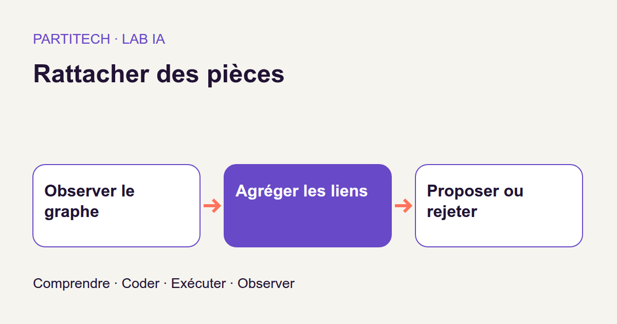
Imagine a back-office screen receiving visit notes to file into case folders. Note O-035 mentions equipment BX-07 and site Cèdre, but no case number. Four case folders are supplied to the application. Which should it suggest to the person doing the filing? More importantly, when is it better to suggest nothing?
If you develop web applications, you may already have solved part of this problem using text searches and joins. But two case folders can have identical wording, and a known equipment relationship does not necessarily provide a certain match.
We will therefore compare several approaches: text alone, a neural network without relationships, then a network using a graph, meaning interconnected objects. We will follow available text and relationships → numerical representations → scores for four candidates → suggestion or abstention.
The aim is to understand what context actually contributes without quietly supplying the answer to recover. A model that still sees the hidden document–case link in its inputs is not solving the problem: it is rereading the solution.
This tutorial produces a suggested association, never an administrative assignment. Data is synthetic. Results describe the r001 protocol, not validation on a company’s documents.
Download the complete project, revision r001
Start from what is actually available
A graph does not necessarily mean a new database
EDM, or electronic document management, organizes documents, metadata and links. In our example, a document is a visit note; a case folder groups information about a case or intervention.
To represent this small world, each object becomes a node: a document, equipment item, site or case folder. An edge is a directed relationship between two nodes. Its type indicates what the relationship means.
For example, we know O-035 — concerns → BX-07 and BX-07 — located at → Cèdre. In relational database terms, these resemble associations between records, with a precise direction and meaning. Using a graph in computation does not mean the Python excerpt installs or requires a graph database: here it manipulates arrays of nodes and relationships.
The link we want to suggest is different: which case folder should document O-035 belong to? It must not already be present among the inputs used to answer.
Observed text and relationships are supplied to the program. The tutorial does not demonstrate automatic extraction of these relationships from a PDF or free-form note.
Rank four candidates, then decide whether to answer
The four candidate case folders are also supplied as input. The program does not select them after consulting the expected folder. This matters: recovering the correct answer among four known candidates is not unrestricted search across an entire EDM system.
Computation produces four scores. The top-ranked folder becomes a suggestion only if its score passes the specified threshold; otherwise, the program abstains.
Take a fictional score example solely to understand this rule: 0.64 ; 0.62 ; 0.21 ; 0.08. With a threshold of 0.60, the first folder is suggested. Yet its score is close to the second’s. The rule described here examines the best score, not the gap between the top two. It therefore does not inherently detect every form of ambiguity.
These four values are not necessarily probabilities summing to 1. A score of 0.64 does not mean ‘a 64% chance this association is administratively correct’. We will return to the difference between a score and a calibrated probability.
An absent relationship is not automatically false
In a real EDM system, a missing link may mean ‘not yet recorded’. It does not necessarily mean ‘this document does not belong to this folder’.
The synthetic corpus provides an experimental advantage: its generator knows which documents have no correct candidate among the four. These cases are called out of scope. They let us check whether the program can reject a request with no correct answer in the proposed list.
Rejection therefore remains local: ‘no good candidate among these four folders’ does not mean ‘no good folder exists in the company’.
Separate whole islands, not just data rows
The corpus contains 80 independent islands. An island is a small group of nodes and relationships sharing no context with the others. The split retains 56 islands for training, 12 for validation and 12 for testing.
Training adjusts network parameters. Validation is used, among other things, to choose thresholds. Testing then measures the selected rule’s behavior without changing it after observation.
Splits share no nodes, edges, equipment or sites. However, words, document types and sentence fragments may remain common. We therefore test new identifiers and graph contexts, not necessarily entirely new vocabulary.
Each island contains four folders. For each, six document links remain visible as context and six others are permanently masked. Four additional documents have no correct candidate folder. The document breakdown is:
| Documents in an island | Calculation from the protocol | Count |
|---|---|---|
| Documents with visible associations | 4 folders × 6 documents | 24 |
| Documents with hidden associations | 4 folders × 6 documents | 24 |
| Documents without a good candidate | Added by the generator | 4 |
| Total documents | 24 + 24 + 4 | 52 |
A caution about the r001 count. The original description states ‘80 independent islands of 52 nodes’ while reporting 5,600 nodes including 4,160 documents. These statements do not agree: 80 × 52 = 4 160, not 5,600. The breakdown above gives 52 documents per island, totaling 4,160 documents. The reported total of 5,600 nodes is retained, but ‘52 nodes per island’ must be checked against the generated corpus. This calculation is not a new count of project files.
For both validation and testing, targets are the 24 hidden-link documents and four out-of-scope documents in each of 12 islands. This gives 12 × 24 = 288 assignable cases and 12 × 4 = 48 out-of-scope cases, totaling 336 targets per split. The 24 visible-link documents in each island remain context: they do not become answers to grade.
Hide the answer in both directions
Suppose a known association is represented both as document → case folder and its inverse case folder → document. Removing only the first edge would leave the same information available in the other direction.
The workflow therefore removes both orientations of each hidden link before inference. Inference simply means using the model to compute a prediction after training.
Degrees, meaning relationship counts used to normalize messages, must also be recalculated. Retaining an old count would preserve a trace of the unmasked graph even after edges are removed. Both neighborhoods and degrees must come from the actually permitted graph.
This precaution does not remove legitimate clues: equipment and sites remain available according to the protocol. It prevents the target relationship from still being supplied, directly or through a calculation performed before removal.
Turn text into vectors with E5
The multilingual-e5-small model, at commit 614241f622f53c4eeff9890bdc4f31cfecc418b3, transforms text into embeddings. An embedding is a list of numbers representing text for similarity calculations. Here, each list contains 384 float32 values, floating-point numbers stored in 32 bits.
These 384 positions are not 384 business fields named ‘site’, ‘equipment’, and so on. They are features learned by the encoder. The encoder produces a numerical representation; it does not write a conversational answer.
Vectors are L2-normalized: each is divided by its length. In a two-dimensional teaching example, [3 ; 4] has length 5 and becomes [0.6 ; 0.8]. Texts are thus compared by representation direction rather than amplitude alone.
Every text receives the literal prefix query: , including folder texts, for this symmetric representation. The E5 documentation for the revision used describes this choice for symmetric tasks and using embeddings as features.
The workflow rejects empty, non-finite or zero means and fails beyond 512 tokens. A token is a text unit handled by the model, not necessarily a whole word. Unlike silently truncating the end, this limit becomes an explicit error.
E5 remains frozen during training: its parameters are unchanged. We learn transformations using its vectors, not a new text encoder. Folder identifiers never become individually learned embeddings; graph indices locate array rows rather than memorize a trainable vector per folder.
Pass along the right context
A graph layer: read neighbors without forgetting your own text
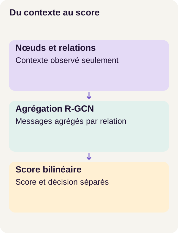
An R-GCN, or Relational Graph Convolutional Network, combines node representations with those of their neighbors while distinguishing relationship types. The original R-GCN paper presents this principle for multi-relational graphs.
The intuition resembles a join followed by grouping: for a destination node, find its neighbors, group their vectors by relationship type and calculate a mean. A learned transformation then processes each mean.
Why retain types? Because ‘concerns equipment’ and ‘is located at a site’ describe different associations. The typed variant can learn different processing. This gives it an additional possibility, not a guarantee of better suggestions.
For each destination and relationship, the layer performs four operations: sum source vectors, divide by the number of corresponding visible edges, apply that relationship’s matrix, then add everything to a projection of the node itself. A ReLU activation finishes the calculation by replacing negative values with zero.
The mechanism can be summarized as new representation = ReLU(transformed node text + transformed neighbor contributions).
Read dimensions before operations
A tensor here is an array of numbers. With N nodes and E observed edges, the first layer handles these dimensions:
| Code object | Shape and meaning |
|---|---|
features |
N × 384: one vector per node |
edges |
E × 3: source, destination, relationship type |
relation_weights |
8 × 384 × 64 in the first typed layer |
| Layer output | N × 64: the same nodes with new vectors |
A matrix is a two-dimensional array. A linear projection combines input values using learned weights to produce a vector of the desired size. Moving from 384 to 64 dimensions does not remove nodes: it changes each node’s representation length.
The project stacks two layers: 384 → 64, then 64 → 64. After one layer, a node can use its direct neighbors’ information; after two, it can also receive information passed through an intermediate neighbor, depending on the orientations actually present. This does not mean instantly reading every path in a large graph.
The executed code: a mean per destination and relationship
Here is the r001 workflow excerpt. Read forward() first, which performs the calculation; we will return to initialization afterward.
import torch
from torch import nn
import torch.nn.functional as F


class RelationalLayer(nn.Module):
    def __init__(self, inputs, outputs, relations, layer, seed=17):
        super().__init__()
        self.self_projection = nn.Linear(inputs, outputs, bias=False)
        self.relation_weights = nn.Parameter(torch.empty(relations, inputs, outputs))
        self.relations = relations
        nn.init.xavier_uniform_(
            self.self_projection.weight,
            generator=torch.Generator().manual_seed(seed + layer),
        )
        for r in range(relations):
            nn.init.xavier_uniform_(
                self.relation_weights[r],
                generator=torch.Generator().manual_seed(seed + 100 + layer * 20 + r),
            )

    def forward(self, features, edges):
        if edges.ndim != 2 or edges.shape[1] != 3 or edges.dtype != torch.long:
            raise ValueError("Edges are source,target,relation integer rows")
        if len(edges) and (
            (edges[:, :2] < 0).any()
            or (edges[:, :2] >= len(features)).any()
            or (edges[:, 2] < 0).any()
            or (edges[:, 2] >= self.relations).any()
        ):
            raise ValueError("Invalid observed edge")
        result = self.self_projection(features)
        for r in range(self.relations):
            selected = edges[edges[:, 2] == r]
            source = selected[:, 0]
            target = selected[:, 1]
            aggregate = torch.zeros_like(features)
            degree = torch.zeros(
                len(features), dtype=features.dtype, device=features.device
            )
            # Every degree and message uses only this currently observed relation.
            aggregate.index_add_(0, target, features[source])
            degree.index_add_(
                0,
                target,
                torch.ones(len(source), dtype=features.dtype, device=features.device),
            )
            aggregate = aggregate / degree.clamp_min(1)[:, None]
            result = result + aggregate @ self.relation_weights[r]
        return F.relu(result)
Input validation requires a two-dimensional edge array with three columns and integer type torch.long. Node indices must correspond to existing rows of features, and relationship indices must fall in the intended range. An edge to a nonexistent node is rejected before participating in computation.
The self-projection starts with self.self_projection(features). Each node thus retains a contribution from its own features even without incoming messages. The option bias=False means this PyTorch linear layer adds no learned constant to its transformation.
Relationship filtering uses edges[edges[:, 2] == r]. For the current type, source gives rows to read and target the destination rows. Other relationships are not mixed into this mean.
Message summation uses aggregate.index_add_(0, target, features[source]). Imagine a GROUP BY destination summing vectors rather than an amount column. When multiple sources share a destination, their values are added into the same row. The _ suffix here indicates that the accumulation tensor is modified in place. The index_add_ documentation details this operation.
A second index_add_ adds 1 values at the same destinations. It obtains degrees for this relationship and this observed graph, not degrees retrieved before masking.
Division turns each sum into a mean. degree.clamp_min(1) replaces zero degrees with 1 to avoid division by zero. This creates no fictional neighbor: an empty sum is still zero, and 0 / 1 remains zero. [:, None] gives degree a column shape to divide every component of a node by the same number.
The relationship transformation uses aggregate @ self.relation_weights[r]. The @ symbol denotes matrix multiplication. The transformed contribution joins the result, then F.relu(result) completes the layer.
The class initializes matrices with Xavier and seeds determined by seed, layer and relationship. A seed fixes a pseudo-random generator’s starting point. It makes initialization controllable; alone, it does not replace all checks needed for reproducible resumption.
A small calculation to check what masking does
Take a two-dimensional teaching example, independent of corpus results. Two neighbors send [2 ; 4] and [6 ; 0] to the same destination through the same relationship.
The sum is [8 ; 4], degree is 2 and mean is [4 ; 2]. If the example’s relationship matrix preserves the first component and doubles the second, its contribution becomes [4 ; 4]. With self-projection [1 ; −1], the sum is [5 ; 3], unchanged by ReLU.
Now remove the second edge. The correct mean is [2 ; 4] / 1 = [2 ; 4]. Reusing old degree 2 would give [1 ; 2]: the representation would still depend on the removed neighbor through its old count.
If every edge is removed, neighbor contributions become zero, but not necessarily the output. This example’s self-projection remains [1 ; −1], then ReLU gives [1 ; 0].
Two further limits are visible in the excerpt. It knows nothing of hidden annotations: target links must have been removed before the call. And it does not deduplicate edges: a repeated row contributes multiple times to the sum and degree. Valid indices therefore do not guarantee the supplied graph’s quality.
Move from vectors to scores, then compare variants
After two layers, the program compares each document representation with each folder’s through a bilinear score. The principle combines two vectors with learned weights to produce a compatibility number. ‘Bilinear’ describes the calculation; it does not mean the business relationship is proven. The excerpt above shows the relational layer, not the complete scoring head or training loop in the ZIP.
Neural decision scores pass through a sigmoid, transforming a raw score into a value between 0 and 1. It equals 0.5 for a zero raw score and increases with it. Its PyTorch definition supplements the mechanism. Applying a sigmoid does not establish that resulting values are reliable association probabilities.
The comparison distinguishes four approaches. E5 cosine directly compares normalized text vectors: it is the text-only reference, not a simple keyword engine. mlp removes edges and retains a network transforming node features. untyped uses edges but collapses all types into one relationship. Finally, typed applies eight distinct relational transformations.
Variants reuse the same candidates, E5 vectors and masks. Their parameter counts are not strictly identical. We therefore compare choices on a specific corpus without automatically attributing every difference solely to relationship typing.
Run every stage in the right order
Prepare the environment
You should be able to read Python, use a terminal and run Docker. Required numerical operations have just been introduced: arrays, means, matrices and scores. Prior graph-network development experience is unnecessary.
Extract the ZIP into a new directory and open a terminal at its root. All following commands run from this folder. Use the project’s intended GPU profile. Before starting, consult its README for resource requirements and installation conditions.
Preflight checks Docker, Compose, the GPU, memory and available space. setup.sh prepares the project; Compose then validates configuration and builds services.
sh scripts/preflight.sh
sh scripts/setup.sh
docker compose config --quiet
docker compose build acquisition tutorial learning inference calibration
Check diagnostics before continuing. An environment error is not resolved by modifying the model or changing thresholds.
Acquire E5, then check real computation inside Docker
The acquisition service downloads nine locked E5 files, checked by size and SHA-256 hash. A hash verifies acquired file identity, not predictive quality.
docker compose run --rm acquisition python scripts/acquire.py --config configs/minimum.yaml
docker compose run --rm tutorial python scripts/check_environment.py
docker compose run --rm tutorial python -m pytest -q
check_environment.py runs E5 inside Docker. Seeing the GPU with nvidia-smi on the host does not prove this containerized computation works. pytest -q then runs project tests. Verify success before continuing: a program test and a suggestion-quality measurement check different things.
Computation services download no drivers and expose no host ports. Setting up a computation environment and running a public API are different topics.
Build data and observe inputs
docker compose run --rm tutorial python -m ged_rattachement_graphe.cli prepare --config configs/minimum.yaml
docker compose run --rm inference python -m ged_rattachement_graphe.cli encode --config configs/minimum.yaml
docker compose run --rm inference python -m ged_rattachement_graphe.cli baseline --config configs/minimum.yaml
docker compose run --rm inference python -m ged_rattachement_graphe.cli inspect-mechanism --config configs/minimum.yaml
prepare builds the corpus. This is the time to check islands, splits and counts, notably the distinction between documents and all nodes. encode calculates E5 vectors. The baseline reference provides a text comparison point, then inspect-mechanism allows examination before training variants.
For a document such as O-035, ask three questions when inspecting inputs: what are the four candidates? Which relationships are visible? Does the link to predict, its inverse or a degree calculated before removal remain? One inspected example often provides more than an aggregate score displayed too early.
Train variants and fix the decision
sh scripts/train_variants.sh
docker compose run --rm calibration python -m ged_rattachement_graphe.cli calibrate --config configs/minimum.yaml
docker compose run --rm tutorial python -m ged_rattachement_graphe.cli evaluate --config configs/minimum.yaml
train_variants.sh runs typed, untyped and mlp. calibrate selects thresholds on validation, then evaluate measures results with that fixed rule.
At each epoch, meaning each training pass over intended examples, three of each training folder’s six visible links are temporarily masked, along with their inverses. The network must learn without the removed link in its immediate context. Permanently hidden links are never reinserted.
Distinguish these mechanisms: temporary masking creates a learning situation from permitted context; permanent masking maintains protocol separation. Neither may be undone to artificially obtain a better prediction.
The project trains for thirty epochs, with four islands per batch. A batch is the group of examples processed in one training step. The AdamW optimizer uses a learning rate of 0.003, weight decay of 0.001 and norm clipping of 1.
An optimizer adjusts weights using gradients, changes in error with respect to those weights. Learning rate controls update magnitude; weight decay reduces weights under AdamW’s rule; clipping limits the norm of excessively large gradients. The AdamW documentation explores the optimizer’s role. These settings identify the experiment; they do not promise success.
Resuming training is more than reloading weights
The workflow interrupts after twelve epochs, then resumes and must exactly recover the continuous path. The checkpoint retains weights, optimizer, sampler determining example order, and random generator states.
Reloading weights alone can produce a model resembling the interrupted one without reproducing its next updates. That is why the check compares states necessary to continue, not just a similar final metric.
This requirement remains environment-specific. The PyTorch reproducibility documentation warns that identical results are not guaranteed across versions and platforms; index_add_ also carries a CUDA caveat. A fixed seed therefore does not establish universal reproducibility. Retain ZIP versions and verify resumption-check results.
Understand the metrics before the numbers
First: is the correct folder ranked well?
Top-1 measures the share of assignable documents whose correct folder ranks first. MRR, or Mean Reciprocal Rank, is the mean reciprocal rank of the correct folder. It is neither the mean rank nor the reciprocal of that mean rank.
If two documents have their correct folders at ranks 1 and 2, Top-1 is 1 / 2 = 0.50. MRR is (1/1 + 1/2) / 2 = 0.75. The reciprocal of the mean rank would give 1 / 1.5, approximately 0.667: a different calculation.
In this tutorial, both measurements concern the 288 documents with a good candidate, even if the threshold later causes abstention on some. They measure ranking, not the number of suggestions sent to a user.
Next: which suggestions are made, and which are correct?
Accepted precision counts correct suggestions among those actually made. Coverage counts suggestions made among the 336 targets, whether correct or not. Rejection recall counts rejected out-of-scope cases among the 48 out-of-scope cases.
Finally, the overall correct-decision rate adds correct suggestions and correct rejections, then divides by 336. Abstaining on a document with a good candidate does not count as a correct decision here.
Take a fictional example of ten documents: eight have a correct folder, two do not. The program makes six suggestions, five correct, and rejects four documents, including both out-of-scope cases.
Its accepted precision is 5/6 ≈ 0.8333, coverage 6/10 = 0.60, rejection recall 2/2 = 1, and overall rate (5 + 2)/10 = 0.70. It perfectly rejects out-of-scope cases but also rejects two documents it could have assigned. A good rejection measure therefore does not describe the whole behavior.
With no suggestions, accepted precision is undefined: there is no denominator. It does not become 1 by convention. Likewise, high coverage does not mean suggested folders are correct.
Choose a threshold without tuning the test afterward
The workflow explores thresholds on validation only. For cosine, the grid runs from −1 to 1 in steps of 0.01. For sigmoid scores, it runs from 0 to 1 in steps of 0.05.
On a tie, the rule retains the value closest to 0 for cosine or 0.5 for sigmoid, then the lower threshold. This tie-breaking is fixed before reading the test. The article does not reproduce calibrate’s full optimization criterion: consult its ZIP implementation rather than inferring an unspecified objective.
Here, calibration means threshold selection. It does not establish probabilistic calibration, which requires checking whether stated confidence levels match observed success frequencies. The scikit-learn probability calibration documentation explains this distinction; it is not an additional stage executed by this project.
Once the threshold is chosen, testing describes this preexisting rule. Changing it because a test figure is disappointing would lose that separation.
Observed results and their scope
Ranking remains identical
Across the 336 test targets, all main variants obtain Top-1 = 0.50 and MRR = 0.75 on the 288 assignable cases. The typed graph therefore does no better than other methods at placing the correct folder first in this reproduction.
Do not confuse this with a complete absence of differences. Suggestion and rejection behavior can change even when ranking does not improve.
Reconstruct the typed graph’s decisions
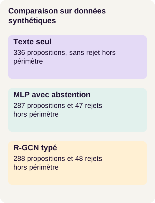
With validation threshold 0.40, typed accepts 288 targets, makes 144 correct suggestions and rejects the 48 out-of-scope cases.
The counts explain metrics without jargon: accepted precision is 144/288 = 0.50, coverage is 288/336 = 0.857143, and overall rate is (144 + 48)/336 = 0.571429. Rejection recall is 48/48 = 1.
The program therefore suggests no wrong folder for the 48 out-of-scope documents, but half of the 288 emitted suggestions remain incorrect. Perfect rejection on this population does not make ranking reliable.
Compare without claiming a graph gain the results do not demonstrate
Cosine uses threshold 0. untyped uses 0.30 and obtains the same counts as typed. Published results do not specify the MLP threshold; the table compares reported decisions without assigning it an additional threshold.
On mobile, scroll the table horizontally.
| Method | Suggestions made | Correct suggestions | Out-of-scope cases rejected, out of 48 | Accepted precision | Overall correct rate |
|---|---|---|---|---|---|
| E5 cosine, text only | 336 | 144 | 0 | 0.428571 | 0.428571 |
mlp, without edges |
287 | 143 | 47 | 0.498258 | 0.565476 |
untyped, single relationship |
288 | 144 | 48 | 0.50 | 0.571429 |
typed, distinguished relationships |
288 | 144 | 48 | 0.50 | 0.571429 |
For cosine, accepting all 336 targets also means suggesting a folder for the 48 documents with no correct one in the list. Its precision is therefore 144/336 = 0.428571. The typed graph improves rejection over this reference here, not Top-1 or MRR.
MLP results are also instructive. With 287 suggestions, it rejects 336 − 287 = 49 documents. Of these, 47 are out of scope, so the other two have a good candidate. This detail is an arithmetic deduction from published counts, not a new analysis of individual predictions.
Its overall rate is explained by (143 + 47)/336 = 0.565476. It is close to the graphs’ rate. We therefore cannot attribute the entire gap from cosine solely to relational context or claim that distinguishing relationship types necessarily improves results.
The takeaway is limited but clear: the studied graphs reject out-of-scope cases better than text alone under this protocol, without ranking correct folders better. These synthetic-data measurements validate neither a business assignment nor the causal contribution of a particular relationship.
Exercise: test the hypothesis before reading the answer
Predict the effect before measuring it
Return to O-035. We have its text and a relationship with BX-07. If this relational channel adds useful information, what should happen when it is removed? Will ranking change? Will fewer suggestions be made? Will rejections improve or worsen?
Write your hypothesis before execution. The effect may be positive, zero or negative. A link that seems intuitively useful does not necessarily improve measured behavior.
Removing a context channel to observe its role is an ablation. Here, the experiment does not simply remove an edge from an already trained model: it trains the no-equipment variant for thirty epochs, with the same candidates and E5 vectors. Its threshold is selected again on validation.
This compares retrained variants, not a last-minute input perturbation of a fixed model. Since text is retained, removing the document–equipment link does not necessarily remove the equipment’s textual mention.
Run the variant and its evaluation
docker compose run --rm learning python -m ged_rattachement_graphe.cli exercise --config configs/minimum.yaml
docker compose run --rm inference python -m ged_rattachement_graphe.cli predict --config configs/minimum.yaml --variant no-equipment --mode continuous
docker compose run --rm calibration python -m ged_rattachement_graphe.cli calibrate-exercise --config configs/minimum.yaml
docker compose run --rm tutorial python -m ged_rattachement_graphe.cli evaluate-exercise --config configs/minimum.yaml
exercise performs the planned experiment, predict produces no-equipment outputs, then calibrate-exercise and evaluate-exercise apply the same validation/test separation. Initial outputs remain hash-protected: the exercise must not quietly overwrite the comparison point.
Compare with supplied observations
In r001 results, no-equipment emits 287 suggestions, 143 correct, and rejects 47 of 48 out-of-scope cases. These counts are close to the initial graph and identical to the MLP counts above. Equal counts do not prove errors concern the same documents: that requires document-by-document output comparison.
You therefore cannot conclude ‘the equipment relationship guarantees the correct folder’. Nor can you conclude it is useless in every EDM system. The result describes this corpus, architecture, training and decision rule.
The answer is to confront your hypothesis with suggestions and rejections, then examine examples. To extend the reasoning by hand, revisit the two vectors in the earlier section: removing an edge must change both numerator and degree. This local check helps explain a leakage source before examining a final score.
Generate figures and check saved states
docker compose run --rm tutorial python lesson/figures/plot.py
docker compose run --rm tutorial python scripts/check_checkpoints.py
Figures complement evaluation; checkpoint checks verify expected workflow states. Retain outputs to study before cleanup below. A curve does not replace inspection of a document, its candidates and visible context.
Troubleshoot, clean up and move toward a product
Distinguish environment failure from model error
The GPU is inaccessible inside Docker? Follow preflight diagnostics, correct the host environment, then retry in a newly extracted folder. Host nvidia-smi status does not replace E5 computation inside the container.
Acquisition fails? Check locked files, sizes and SHA-256 hashes. Do not substitute another model or revision to make the error disappear: that would change experiment conditions.
A checkpoint check fails? Keep material useful for diagnosis. Supplied cleanup deletes only outputs; it neither repairs nor replaces retained checkpoints. For a fresh full workflow, a new extraction avoids mixing states from multiple attempts.
Before cleanup, copy results and figures to retain. The following commands stop the project, display and delete only outputs, then end the workflow. Data, models and checkpoints remain. No global Docker cleanup is needed.
docker compose down
docker compose run --rm tutorial python scripts/clean.py --outputs-only
docker compose down
Understand what isolation provides
Services use the user’s UID and GID, their system identifiers. Their root filesystem is read-only; only areas needed for each service’s role are mounted writable. The project removes extra Linux capabilities, uses no-new-privileges, sets CPU, memory and process limits, and provides temporary space in tmpfs.
Acquisition can access locked public files. Computation services run with networking disabled. This separation helps keep the workflow within its intended scope; it is not a security certification against a Docker administrator.
From a score to a review interface
In a real application, start by defining with business teams what a correct association means, which documents are involved and where candidate folders come from. Build representative annotations and evaluation before replacing the fictional corpus.
Permissions must apply before scoring: first place in a ranking does not authorize displaying a confidential folder. You must also decide what to do when no authorized folder is available, whereas the tutorial always supplies four.
Workflow ties are broken by identifier to stabilize computation. This choice has no business meaning. If two candidates tie, a smaller identifier does not make one more relevant.
A review interface can present the document, candidates, consulted relationships and suggestion, then let a person confirm, reject or correct it. This is a product idea to develop, not an interface already supplied by the excerpt. The subgraph shows available context; it is not a causal explanation of the association’s validity.
Authentication, APIs, persistent storage, suggestion logging, monitoring, backups, load tests and business evaluation remain to be planned. Version graph, data, decision rules and model together. A suggestion must be retrievable and challengeable, not merely displayed then forgotten.
This tutorial workflow changes no folder or permission. Automating an administrative action would be a different scope to define and validate.
Summary
We started with a back-office question: suggest a folder from a note and known relationships. E5 turns text into frozen vectors; the relational network combines them with permitted neighbors; the score ranks four candidates; a separate rule decides whether to suggest or abstain.
The essential check lies in the inputs: remove the target link and inverse, recalculate degrees and separate islands. Otherwise, an impressive metric may simply measure the answer’s presence in context.
The numbers then show why objectives must be separated. In this reproduction, the graph improves out-of-scope rejection over cosine, but not folder ranking. The edgeless model remains close, and relationship typing demonstrates no gain on published metrics.
You now have a workflow for learning to represent context, verify aggregation and interpret a decision. The next step is not turning scores into certainty: it is evaluating what remains wrong on the documents and uses actually targeted.
Primary sources and further reading
The workflow’s original references are the R-GCN paper, the E5 documentation for the acquired revision and the PyTorch 2.8 index_add_ documentation.
Supplementary links throughout the text expand on linear projections, sigmoid, AdamW, reproducibility and probabilistic calibration. They explain concepts; they add no new training or measurements to r001. To reproduce it, retain ZIP versions and commands rather than replacing them with current documentation examples.