





Imagine a manufacturer's document portal. You already have the back office, manuals and access permissions. You would now like to use these texts with a language model, but machine references and technical vocabulary do not always resemble what it encountered during its initial training.
One approach is to have it study the manuals. Not by asking it to read them in a prompt, but by continuing its training: we hide some parts of the text, then ask it to recover them.
This resembles a fill-in-the-blanks exercise. The interesting challenge comes next: does the model improve on manuals without getting worse on other texts? And how can we tell if the blanks change at every evaluation?
In this tutorial, we will adapt BERT to a domain, compare a variant with regular review of a control corpus, then measure both effects using the same exam for every model. The manuals are synthetic: we are studying a learning mechanism, not a maintenance assistant ready for deployment.
Download the complete tutorial project
What we are building
The project compares three states of the same model. The baseline is the model before our adaptation. The second path continues its learning on domain documents. The third adds replay: blocks from the control corpus periodically return in training batches.
A checkpoint is a saved model state; resuming training also requires the other states needed for computation. We will return to this distinction when discussing resumption.
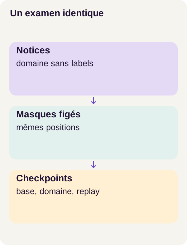
Before comparing these checkpoints, the program prepares the same evaluation texts and the same positions to predict. It then measures two things, separately for domain and control: the probability assigned to expected tokens, summarized by NLL, and how often the model's top choice is correct, called top-1 accuracy.
By the end, you will be able to follow the path text → tokens → partially corrupted input → predictions → metrics. You will also know how to distinguish improvement on this exercise from an ability to answer a business question correctly. The program builds neither the portal mentioned in the introduction nor an industrial decision-making system.
Concepts explained
A token is not necessarily a word
The model does not receive a Python string directly. A tokenizer splits text into vocabulary units, called tokens, then assigns numeric identifiers to them. A unit can represent a word, a word fragment or a symbol. In this project, we work with subword IDs.
Think of it as converting representations: your application handles text; the model handles arrays of integers. An ID identifies a vocabulary entry. Its numeric value alone does not indicate the token's meaning.
The variant used is google-bert/bert-base-uncased. Its official model card specifies that it was pretrained in English and does not distinguish uppercase from lowercase. The original article's French explanations change neither this model nor the reference data.
Learn with a fill-in-the-blanks exercise
A masked language model, or MLM, tries to recover tokens from their context. BERT can use text before and after the position to predict. It therefore does not perform the same task here as a model that must only write a continuation of a text. This principle is described in the BERT paper and the Hugging Face MLM guide.
To illustrate the idea, imagine this sentence with a blank: “The documented temperature is [MASK] degrees.” This illustrates the mechanism, not a measured output or actual BERT tokenization.
But where do we find the correct answer, since the manuals are unlabeled? In the original text, before modifying it. The program retains the expected token's identifier, then alters its position in the input. It thus automatically creates both the example and its answer key: this is self-supervised learning.
“Without manual labels” therefore does not mean “without learning targets.” Here, nobody needs to annotate every sentence with a category; the original tokens act as labels.
What training changes
At each position, the model produces logits: scores for possible tokens. Softmax turns these scores into a probability distribution. The loss penalizes the model when it assigns too little probability to the reference token.
Backpropagation computes gradients, meaning the sensitivity of this loss to the network's parameters. The optimizer uses these gradients to change the weights, the learned numbers determining the model's behavior. A batch groups several examples processed in one computation.
We do not start again from random weights: BERT already has initial training. We continue a language objective on a specialized corpus. This is domain adaptation through continued pretraining, studied notably in Don't Stop Pretraining.
This is not yet supervised training to answer technical questions. Recovering a token in a manual and selecting a correct procedure in response to a request are different tasks. The tutorial measures only the first.
Adapt without betting everything on the new domain
By training the model on manuals, we change weights that also contributed to its predictions on other texts. Its results can therefore improve here and deteriorate elsewhere.
Catastrophic forgetting refers to this loss of performance as new learning proceeds. In our experiment, we observe a narrower indicator: possible deterioration on the chosen control corpus. We do not measure all of BERT's prior knowledge.
Replay acts as interleaved revision: instead of working only on the new subject, training also encounters control examples. It neither restores old weights nor queries a second model. In r1, this variant changes the batch schedule, not the MLM principle.
Finally, the comparison must use the same exam. For a web developer, the analogy is a regression test suite: changing test cases at the same time as the implementation prevents us from isolating what caused a score change.
Docker and GPU prerequisites
You should be able to read Python functions, lists, dictionaries and JSON, and use a terminal with Docker. The necessary learning concepts are explained in the walkthrough.
The r1 reproduction uses Linux x86_64, Docker Compose, NVIDIA Container Toolkit and one 24 GiB RTX 3090. Allow 16 GiB of RAM and 16 GiB of disk space, excluding shared Docker layers. These are project provisions, not measured minimums; no CPU walkthrough is validated here.
locks/models.lock.json pins google-bert/bert-base-uncased to revision 86b5e0934494bd15c9632b12f734a8a67f723594. locks/environment.lock.json describes the environment. Like a dependency lockfile in a web project, these files identify the recipe used: do not replace a version to silently make an error disappear.
The acquire service downloads public assets. The gpu service performs local computations without networking. The check_environment.py script initializes CUDA, NVIDIA's computing environment, from inside the container. A card visible on the host is not enough; Docker must also be able to use it. The Docker Compose GPU guide explains this integration.
Data and the central function
What will we actually count?
A corpus is a collection of documents. A split is a partition of that collection: training changes the model, validation tracks development choices, and testing provides final evaluation. Domain and control each have validation and test splits.
Here are the counts retained in r1 evaluation. These are supervised positions, meaning tokens on which the score is calculated, not document or question counts.
| Split | Evaluated tokens | Role |
|---|---|---|
domain-validation |
3,089 | Track domain adaptation |
domain-test |
3,054 | Measure the final domain result |
control-validation |
1,318 | Track effects on the control |
control-test |
1,233 | Measure the final control result |
All three checkpoints receive the same positions and corrupted inputs for each split. The term “masked tokens” is shorthand: we will see that some evaluated positions remain visible in the input.
An r1 corpus example has the identifier domain-006-0. It is a fictional Velon manual about a pump coupling: it asks for the pump to be isolated before inspection and mentions a documented operating temperature of 62 degrees. This information belongs to the exercise data. It is never an instruction for real equipment.
Freeze the questions and their answer key
The following continuous excerpt from src/domain_mlm/eval_masks.py builds the comparison set, then checks that it remains identical.
def freeze_evaluation_masks(config):
    tokenizer = AutoTokenizer.from_pretrained("models", local_files_only=True)
    generator = torch.Generator().manual_seed(config["seed"] + 1000)
    sets = {}
    for corpus in ("domain", "control"):
        for split in ("validation", "test"):
            key = corpus + "-" + split
            rows = read_json("outputs/" + key + ".json")
            ids = torch.tensor([r["input_ids"] for r in rows])
            masked, labels, _ = mask_tokens(
                ids, tokenizer, generator, config["mask_probability"]
            )
            sets[key] = [
                {
                    **row,
                    "original_ids": row["input_ids"],
                    "input_ids": masked[i].tolist(),
                    "labels": labels[i].tolist(),
                }
                for i, row in enumerate(rows)
            ]
    target = Path("outputs/eval-masks.json")
    if target.exists():
        assert read_json(target) == sets, "Evaluation masks changed"
    else:
        save_json(target, sets)
Let's start with what this function does not do: it does not call BERT to predict tokens or launch training. It prepares the examples that will later be sent to models.
AutoTokenizer.from_pretrained("models", local_files_only=True) loads the tokenizer already acquired in the local directory. Here, models is a path, not an automatic download request.
torch.Generator().manual_seed(config["seed"] + 1000) creates a dedicated pseudorandom generator. The seed sets the starting point of its sequence of draws. The + 1000 offset is a project choice: it does not mean “one thousand masks.”
The two loops successively traverse domain-validation, domain-test, control-validation and control-test. torch.tensor(...) turns the lists of IDs into a numerical array, or tensor. This construction assumes rows of compatible length; the excerpt does not itself adjust their lengths.
After mask_tokens, each row retains its metadata through **row, then three complementary representations: original_ids for tokenized text before transformation, input_ids for the corrupted input, and labels for targets to recover. tolist() makes tensors saveable as JSON.
Finally, outputs/eval-masks.json is created if absent. If it exists, the code reconstructs the expected data and compares it in full with the saved content. A difference triggers Evaluation masks changed rather than silently overwriting the old exam. The r1 walkthrough also specifies a lock and target counts per split; their additional writing does not appear in this excerpt.
Same seed and same masks: two different guarantees
The generator is shared by all four splits and advances with every draw. Changing row order, row length or the number of draws can therefore change the resulting sequence, even with the same initial seed. Comparing the file protects the data actually prepared, not merely a configuration value.
This protection has an explicit limitation: it uses assert. Python can disable assertions in optimized mode, notably with the -O option. Keep the walkthrough's execution mode; in a production adaptation, a mandatory check should not rely on assertions that can be disabled. This is the behavior described in the Python documentation, not a change to the code above.
Freezing masks eliminates one source of variation, not all the others. You must still retain the tokenizer, data, evaluation settings and environment. PyTorch notes that the same seed does not guarantee identical results across all platforms or versions.
Create an input and MLM targets
The lock describes the exam. The continuous excerpt from src/domain_mlm/collator.py now describes the mechanism creating inputs and targets, also used during training.
def mask_tokens(input_ids, tokenizer, generator, probability=0.15):
    if not 0 <= probability <= 1:
        raise ValueError("Mask probability out of range")
    eligible = torch.ones_like(input_ids, dtype=torch.bool)
    for value in tokenizer.all_special_ids:
        eligible &= input_ids != value
    chosen = (torch.rand(input_ids.shape, generator=generator) < probability) & eligible
    labels = input_ids.clone()
    labels[~chosen] = -100
    corrupted = input_ids.clone()
    choice = torch.rand(input_ids.shape, generator=generator)
    corrupted[chosen & (choice < 0.8)] = tokenizer.mask_token_id
    admissible = torch.tensor(
        [i for i in range(len(tokenizer)) if i not in tokenizer.all_special_ids]
    )
    random_ids = admissible[
        torch.randint(len(admissible), input_ids.shape, generator=generator)
    ]
    random_positions = chosen & (choice >= 0.8) & (choice < 0.9)
    corrupted[random_positions] = random_ids[random_positions]
    return corrupted, labels, eligible
The first step is to distinguish what can be selected from what actually was selected.
eligible is a boolean array with the same shape as the IDs. The loop excludes the tokenizer's special tokens, such as start, separator or padding markers. Padding fills out short sequences to form arrays of the same width; it does not represent text to recover.
chosen then applies a random draw at every position and combines it with eligible. The probability parameter defaults to 0.15 in this function. When freezing evaluation, the caller passes config["mask_probability"]: consult the locked configuration for the walkthrough's actual value.
labels starts as a copy of the original tokens. Unselected positions become -100. Under the PyTorch cross-entropy contract, this value marks a target to ignore. It does not replace text in the model's input. An unsupervised token can still help recover its neighbor through context.
The code then creates corrupted, an independent copy of the input. For selected positions, a second draw determines the transformation: below 0.8, the token becomes the mask marker; between 0.8 and 0.9, it is replaced with an admissible random token; from 0.9 onward, it remains unchanged.
We therefore obtain 80% mask, 10% random replacement, 10% unchanged among selected positions. These are probabilities, not exact quotas imposed on every batch. With a 15% selection probability, expected proportions among eligible positions are respectively 15% × 80% = 12%, 1.5% and 1.5%.
One detail matters: admissible excludes special IDs, but not each position's original ID. A random draw can therefore land on the original token. Seeing an unchanged input is not enough to determine which branch was drawn.
Follow one row without loading BERT
Here is a teaching example built by hand with fictional IDs. It does not use BERT's actual vocabulary or come from r1 results. We select three positions to show the three branches; we are not trying to reproduce their frequencies with such a short row.
| Position | Original ID | Eligible? | Selected? | ID given to the model | Label | Explanation |
|---|---|---|---|---|---|---|
| 0 | 1, start | No | No | 1 | -100 | Special marker |
| 1 | 7 | Yes | Yes | 3, mask | 7 | The model must recover 7 |
| 2 | 8 | Yes | Yes | 12 | 8 | Replacement does not change the answer key |
| 3 | 9 | Yes | Yes | 9 | 9 | The token remains visible but is evaluated |
| 4 | 10 | Yes | No | 10 | -100 | Visible context, no direct target |
| 5 | 2, separator | No | No | 2 | -100 | Special marker |
| 6 | 0, padding | No | No | 0 | -100 | Padding |
There are three targets, but only one mask marker. Counting only occurrences of [MASK] would therefore give the wrong denominator for the metric. Here, targets are identified by labels != -100.
Similar names can be confusing: eligible indicates candidate masking positions; chosen indicates supervised positions; an attention mask, meanwhile, indicates positions the network can use as context. The function shown does not return an attention mask: it returns corrupted, labels and eligible.
One final case to know before modifying the program: the function accepts zero probability and does not force every batch to contain a target. At probability=0, all labels are -100. A mean-loss computation must explicitly handle a batch without targets rather than treating it as perfect learning. This excerpt does not show the training policy for that case; this does not mean it occurred in r1.
Install, check and freeze the exam
Prepare the environment
Extract the ZIP and open your terminal in its root directory. All the following commands run from that folder. They retain the order of the r1 walkthrough described in README.md and lesson/tutorial.json.
sh scripts/setup.sh
docker compose config --quiet
docker compose build acquire gpu
docker compose run --rm acquire python scripts/acquire.py --config configs/minimum.yaml
docker compose run --rm gpu python scripts/check_environment.py --config configs/minimum.yaml
docker compose run --rm gpu python -m pytest -q
setup.sh prepares the project. docker compose config --quiet checks that the Compose configuration is usable, then build builds the service images. Acquisition retrieves assets according to the locks; the environment check verifies CUDA inside the container; pytest runs the program's tests.
Wait for these steps to finish without errors before training. A passing test suite checks the mechanisms it covers; it does not yet tell us whether adaptation will be useful.
Prepare documents and preserve the exam
docker compose run --rm gpu python -m domain_mlm.cli prepare --config configs/minimum.yaml
docker compose run --rm gpu python -m domain_mlm.cli inspect-mask --config configs/minimum.yaml
docker compose run --rm gpu python -m domain_mlm.cli freeze-eval --config configs/minimum.yaml
prepare creates the walkthrough's data. inspect-mask lets you observe their transformation: connect original IDs, corrupted input and labels. In particular, find an ignored position and a selected position; they play different roles.
freeze-eval then prepares the four frozen evaluation splits. In outputs/eval-masks.json, check for their names and the original_ids, input_ids and labels fields. Target counts must match the table above.
Freezing takes place before the training runs we want to compare. It prevents quietly replacing a difficult exam with a more favorable one. Checkpoint changes can then be compared on the same inputs, provided the rest of the protocol is also retained.
Adapt, resume and measure
We can now run adaptation alone, then adaptation with replay. The following commands also test interruption and resumption before producing final measurements.
docker compose run --rm gpu python -m domain_mlm.cli train --config configs/minimum.yaml
docker compose run --rm gpu python -m domain_mlm.cli train --config configs/minimum.yaml --variant replay
docker compose run --rm gpu python -m domain_mlm.cli train --config configs/minimum.yaml --stop-after 150 --run-name interrupted
docker compose run --rm gpu python -m domain_mlm.cli train --config configs/minimum.yaml --resume artifacts/checkpoints/interrupted/state.pt --run-name resumed
docker compose run --rm gpu python -m domain_mlm.cli compare-resume --config configs/minimum.yaml
docker compose run --rm gpu python -m domain_mlm.cli evaluate --config configs/minimum.yaml
docker compose run --rm gpu python -m domain_mlm.cli inspect-cases --config configs/minimum.yaml
Read the commands as an experiment
The first train command follows the domain-adaptation path. The second selects --variant replay. According to the r1 description, this variant changes only the batch schedule: it introduces control review into learning. It is neither a second type of model nor a new metric.
Both variants must then be compared against the unadapted baseline on domain and control. Looking only at manuals would be like checking a new feature while forgetting tests for existing features.
Resuming is more than reloading weights
The command with --stop-after 150 --run-name interrupted produces the stop planned by the walkthrough. The next resumes artifacts/checkpoints/interrupted/state.pt under the name resumed. Keep this order: the file must exist before it is read.
Why not simply reload the model and start again? Because a training trajectory also depends on optimizer state and random draws. The RNG, or pseudorandom number generator, must resume at the point reached, not necessarily at the start of its sequence. The torch.Generator documentation specifically distinguishes the initial seed from saved state.
The interrupted, resumed and compare-resume steps check this full resumption in r1. They should not be interpreted as additional training intended to improve the score. Consult the result of compare-resume to verify this property in your run.
Finally, evaluate produces metrics, then inspect-cases shows examples. This order is useful: cases explain an aggregate measurement; they do not replace it. For a given manual, compare the expected token, predictions and their probabilities; do not select only the most convincing case.
Metrics before measurements
NLL: how much probability does the correct answer receive?
NLL stands for negative log-likelihood. For one evaluated position, if the model assigns probability p to the original token, its contribution is:
NLL for the position = -ln(p)
ln is the natural logarithm. You do not need to memorize its values: remember that assigning more probability to the expected token reduces the penalty. A very low probability costs much more than moderate uncertainty. The natural logarithm expresses this loss in nats, not percentages.
The following table is a three-candidate teaching example, independent of BERT and r1 measurements. “Other” represents a single third candidate here; every row sums to 1.
| Fictional situation | Expected token probability | Main competitor | Other | Correct top-1? | Approximate NLL |
|---|---|---|---|---|---|
| A | 0.20 | 0.75 | 0.05 | No | 1.6094 |
| B | 0.40 | 0.50 | 0.10 | No | 0.9163 |
| C | 0.60 | 0.35 | 0.05 | Yes | 0.5108 |
| D | 0.90 | 0.07 | 0.03 | Yes | 0.1054 |
From A to B, the top choice remains wrong, but the expected token's probability rises: NLL improves. From C to D, the top choice remains correct, and NLL still distinguishes the two distributions. Top-1 accuracy therefore does not tell everything that probabilities tell us.
Over a corpus, we add contributions and divide by the number of supervised positions. Other positions, notably those whose label is -100, must not dilute this average.
Take another fictional calculation: one block contributes one target with NLL 2, and another contributes three targets with average NLL 0.5. The per-token mean is (2 + 3 × 0.5) / 4 = 0.875. The unweighted mean of the two blocks would be (2 + 0.5) / 2 = 1.25, a different quantity. The unit specified here really is the evaluated token, not the document or batch.
Top-1 accuracy: is the first choice correct?
For each supervised position, we retain the token with the highest probability and compare its ID with the reference ID.
top-1 accuracy = number of correctly predicted tokens / number of evaluated tokens
Three correct predictions out of four give 3 / 4 = 0.75, or 75%. That does not mean that three documents out of four are fully understood, nor that three business answers out of four would be correct.
The answer key remains the original token. Another plausible token gets no credit just because a person might find the sentence acceptable. Likewise, correctly predicting part of a word does not guarantee that the entire word or sentence is correct. These conventions make the measure precise, but limit how it can be interpreted.
The forgetting indicator: a signed difference
The control_test_forgetting_nll field measures:
variant NLL on control-test - reference NLL on control-test
A positive value means that NLL increased: the variant performs less well on this control exercise. A negative value means an improvement. Zero means the two average NLL values are equal; it does not prove that every prediction is identical.
Fictional example: if the reference is 2.0 and the variant is 2.6, the indicator is +0.6. With a variant at 1.7, it is -0.3. These differences are neither percentages nor counts of knowledge lost.
An NLL increase can be substantial while top-1 changes little: the model may keep many first choices while sharply reducing target probabilities at a few positions. The two metrics are complementary.
Actual results and what we learned
The following numbers are from reproduction r1, using the synthetic corpus and fixed masks described above. They are not the calculation examples from the previous section.
| Model state | Top-1 on domain-test |
Top-1 on control-test |
control_test_forgetting_nll |
|---|---|---|---|
| Unadapted reference | 0.3850687622789784 | 0.46228710462287104 | 0, by definition of the difference |
| Domain adaptation alone | 0.9747871643745907 | 0.45093268450932683 | +0.6229252393711704 |
| Adaptation with replay | 0.9754420432220039 | 0.9772911597729116 | -2.7341342250796132 |
The table gives NLL differences, not absolute values. Without the reference NLL, these differences cannot be used to reconstruct the three losses. Keep this distinction in mind when reviewing the output produced by evaluate.
Adaptation alone improves the manuals, but regresses on the control
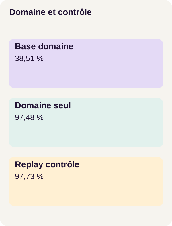
As a percentage, domain top-1 rises from around 38.51% to 97.48%. On the control, it moves from around 46.23% to 45.09%, a drop of about 1.14 percentage points. The +0.6229252393711704 NLL indicator also describes a deterioration in control performance, on another scale.
We can make these proportions concrete. By multiplying the reported rates by the target counts, we obtain 1,176 then 2,977 correct tokens out of 3,054 for the domain, and 570 then 556 out of 1,233 for the control. These are counts calculated from the measurements, not new inferences.
The result therefore demonstrates the expected trade-off: improving performance in a new domain does not guarantee preserving performance elsewhere.
Replay improves both scores in this experiment
With replay, the domain reaches around 97.54%, or 2,979 correct tokens out of 3,054; the control reaches around 97.73%, or 1,205 out of 1,233. The negative NLL indicator also shows an improvement in the control relative to the reference.
In the domain, the gap between adaptation alone and replay amounts to two additional correct tokens, or about 0.0655 percentage points. This puts the many decimal places in the table into perspective: they are not evidence of general superiority or statistical significance.
On the control, replay does more here than preserve the initial level: it improves it substantially. This finding belongs to this synthetic corpus. We cannot infer that the model has preserved all of its general capabilities, or that it can correctly answer a user's question.
What freezing the masks does not prove
Identical examples make the comparison easier to read. By themselves, they do not demonstrate that training and evaluation data do not overlap, nor that formulations are diverse.
The r1 description indicates replay of the control corpus, but the two excerpts shown do not specify either the reinjected IDs or replay frequency. To audit this boundary, read the ZIP configuration and batch program. When adapting to your own data, reserve separate control partitions for replay and for evaluation: training on the test control and then scoring it would be a different protocol.
This is not a finding of leakage in r1. It distinguishes what the masking code visible here verifies from what must be checked elsewhere in the project.
The main lesson is therefore not “replay solves forgetting.” It is more useful: measure domain learning and regressions on a control together, then retain the evidence needed to understand their differences.
Exercise: predict, then run
Imagine two checkpoints evaluated with independently sampled masks. The first must recover common words; the second must recover rare technical references. Is a score difference enough to attribute an improvement or regression to the model?
Before running the command, write down your answer to that question, then to this one: could the score change even if we used exactly the same checkpoint twice?
A small hand-built counterexample helps formulate the hypothesis. Suppose a fixed model correctly recovers positions A and B, but not C and D. An exam covering A and B gives 100%. Another covering C and D gives 0%. The weights did not change: only the questions changed. This is not BERT output, but it demonstrates the comparison pitfall.
Now run the provided exercise:
docker compose run --rm gpu python -m domain_mlm.cli exercise --config configs/exercise.yaml
Compare its output with the fixed-mask set. The expected explanation is not that every mask change necessarily changes the score: it may make no difference. The problem is that it introduces an additional cause that the score alone cannot separate from the checkpoint's effect.
Conversely, a fixed exam must not become a set of answers on which we endlessly tune our parameters. Validation supports development choices; the test remains reserved for the final assessment. To study masking variability in a separate experiment, one option would be to prepare several exams in advance and administer each one to every checkpoint. This extension is not run in the pathway presented here.
Finish with the figures, checkpoint check, cleanup preview, and project shutdown:
docker compose run --rm gpu python lesson/figures/plot.py
docker compose run --rm gpu python scripts/check_checkpoints.py
docker compose run --rm gpu python scripts/clean.py --scope generated --dry-run
docker compose down --remove-orphans
--dry-run displays what cleanup would target, but does not delete any results. Stopping Compose does not replace preserving the JSON files and checkpoints needed to review your experiment.
Adaptation, production, troubleshooting, and cleanup
Replacing the synthetic corpus without losing the comparison
Start by defining the capabilities the model must acquire and those it must retain. A control corpus that is useful for your application must represent the latter; it is not automatically a sample of everything initial pretraining had taught.
Version documents, the tokenizer, partitions, and masks. In a new experiment, also isolate similar documents or versions of the same manual so that a test does not merely retrieve wording that was almost seen in training. This recommendation completes the protocol; the two excerpts presented do not detail any audit of document similarity.
Choose settings on validation, while keeping a record of the replay interval and origin. Set acceptance thresholds for both domain and control before delivery. Do not reduce the comparison to a single successful example or to domain NLL alone.
For French or multilingual texts, do not assume that the locked English variant meets the same need. Changing the tokenizer or model creates a new experiment: token counts and granularity may change, so an NLL per token is no longer directly comparable with r1.
Moving from token predictions to an application
The project adapts a masked language model. It does not validate a question-answering system, an instruction extractor, or a maintenance decision. These uses require their own reference data, error criteria, and evaluations by domain experts.
For business documents, govern access, sensitive information, and retention of artifacts. A manual completed correctly in an exercise does not become an approved procedure. The Velon case and its 62 degrees remain fictional data, not an operational instruction.
Diagnose without silently changing the experiment
CUDA fails. Run check_environment.py again, then check the container's GPU access with the NVIDIA Container Toolkit guide. Do not change the model to solve an environment problem.
Acquisition fails. Restore the acquire service's network, then rerun its command. Keep the model and dependency locks; another revision would not constitute the same reproduction.
Evaluation masks changed appears. Compare the prepared data, their order, the configuration, and the tokenizer with those from the initial freeze. Do not delete the old file to make the check pass: you would lose your comparison baseline. An intentional change requires a separate experiment and a new freeze, not an invisible replacement.
The resume checkpoint is missing. Check that the interrupted command completed and produced the expected file before starting resumed. The existence of any weights file does not replace the complete state required by this command.
Finally, docker compose down --remove-orphans stops the project services without deleting the outputs described here. clean.py --dry-run only announces its targets. Preserve your results before undertaking different cleanup.
Official sources
The measurements, paths, commands, and two code excerpts above belong to the downloadable r1 pathway. The following references provide further detail on the mechanisms; they are not the source of its scores and do not replace its locked versions.
- Hugging Face: masked language modeling tasks and BERT base uncased: the MLM objective and model used.
- Devlin et al.: BERT and Gururangan et al.: Don't Stop Pretraining: context for bidirectional representation and adaptation through pretraining.
- PyTorch: cross entropy, versioned CrossEntropyLoss reference, random generators, and reproducibility: ignored targets, random state, and the limits of guarantees.
- Python: assert statement, Docker Compose: GPU support, and NVIDIA Container Toolkit: execution checks and environment.