





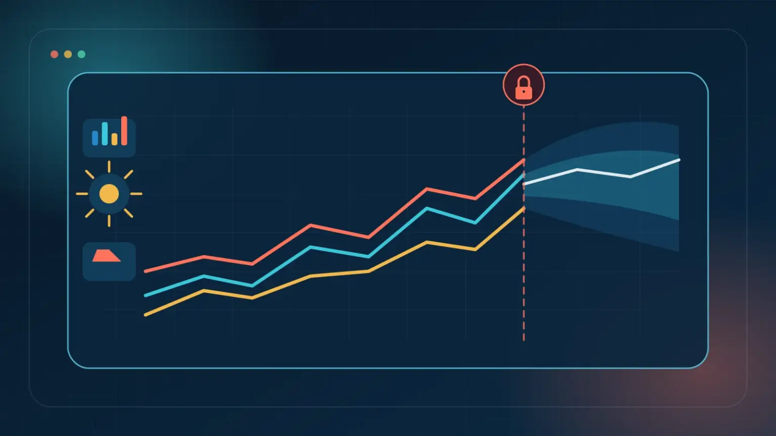
On 31 August 2026, Google Research presented TimesFM-3, a zero-shot foundation model designed for multivariate time series. The publisher reports 330 million parameters, pretraining on more than one trillion time points, and native support for multiple targets as well as historical or future-known variables. These capabilities make the model interesting for accelerating forecasting projects. They do not remove the need for local comparison, data analysis, or a governance framework.
Key takeaway: TimesFM-3 should be treated as one additional candidate, not as a universal truth. A serious pilot compares it with a naïve baseline, a statistical model, and the approach currently in use, on reproducible time windows and metrics connected to business decisions.
1. What TimesFM-3 really brings
The first versions of TimesFM focused on univariate forecasts: the model observed the history of one series and predicted what came next. TimesFM-3 adds a multivariate representation. It can forecast several related series and use variables that influence the phenomenon.
Google distinguishes three families of inputs. Targets are the series to forecast, such as sales for several products. Past covariates are known only in the historical record, such as observed traffic. Dynamic covariates are known over the future horizon, for example a promotion calendar, public holidays, or a weather forecast available when the decision is made.
The architecture alternates causal temporal attention with attention across variables. The model produces the entire horizon in a single non-autoregressive pass and provides nine quantiles between the 10th and 90th percentiles. This probabilistic output represents several scenarios rather than a single line.
Google reports an average first place across several public benchmarks against other pretrained models. These are results communicated by the design team, using defined datasets and protocols. They indicate potential, but do not predict performance on your series, your breaks in trend, your granularities, or your operational constraints.
2. Why zero-shot changes how a project starts
A zero-shot model can be applied without specific training for each series. This property reduces the time needed to obtain an initial reference. A team can load its history, define the horizon, and quickly compare the result with its existing methods.
This gain is particularly useful when an organization has many short or heterogeneous series: sales by distribution point, ticket volumes by category, infrastructure consumption by service, or stock requirements by item. Training and maintaining a separate model for every series becomes expensive.
Zero-shot does not mean “no data work”. You still need to define the frequency, handle gaps, distinguish real zeros from missing values, process scope changes, and choose the relevant history period. A powerful model cannot infer that a store closed, a sensor changed, or an accounting rule moved the volumes.
Inventory, quality, permissions, and traceability must therefore come before choosing the model, as in our guide to preparing your data for a generative AI project. For forecasting, add the actual availability date of each variable to this foundation.
You must also compare total time. The model may avoid a training phase while requiring more inference compute or specific infrastructure. The relevant cost is that of a forecast that is produced, supervised, and used, not only that of the initial notebook.
3. Where multivariate forecasting can create value
Multivariate forecasting is useful when the series genuinely share a dynamic. Sales of complementary products, the loads of several platform services, or the volumes of branches subject to the same calendar can inform one another.
Variables known in the future are often even more important. A promotion calendar, a planned closure, a launch, a public holiday, or an already recorded reservation can change the horizon. A univariate approach sees the past effect but ignores the upcoming event; a model that accepts these covariates can incorporate it.
Quality nevertheless depends on the stability of the relationship. A promotion does not always have the same effect depending on price, channel, availability, or season. A weather forecast itself contains uncertainty. Adding more variables does not guarantee better generalization and can create dependence on data unavailable in production.
Before the pilot, build a simple matrix: variable, availability at forecast time, update frequency, historical quality, owner, and business rationale. Any variable unknown at the actual decision time must be excluded from the future dataset, even if it is present in the warehouse afterwards.
4. Avoiding leakage between past and future
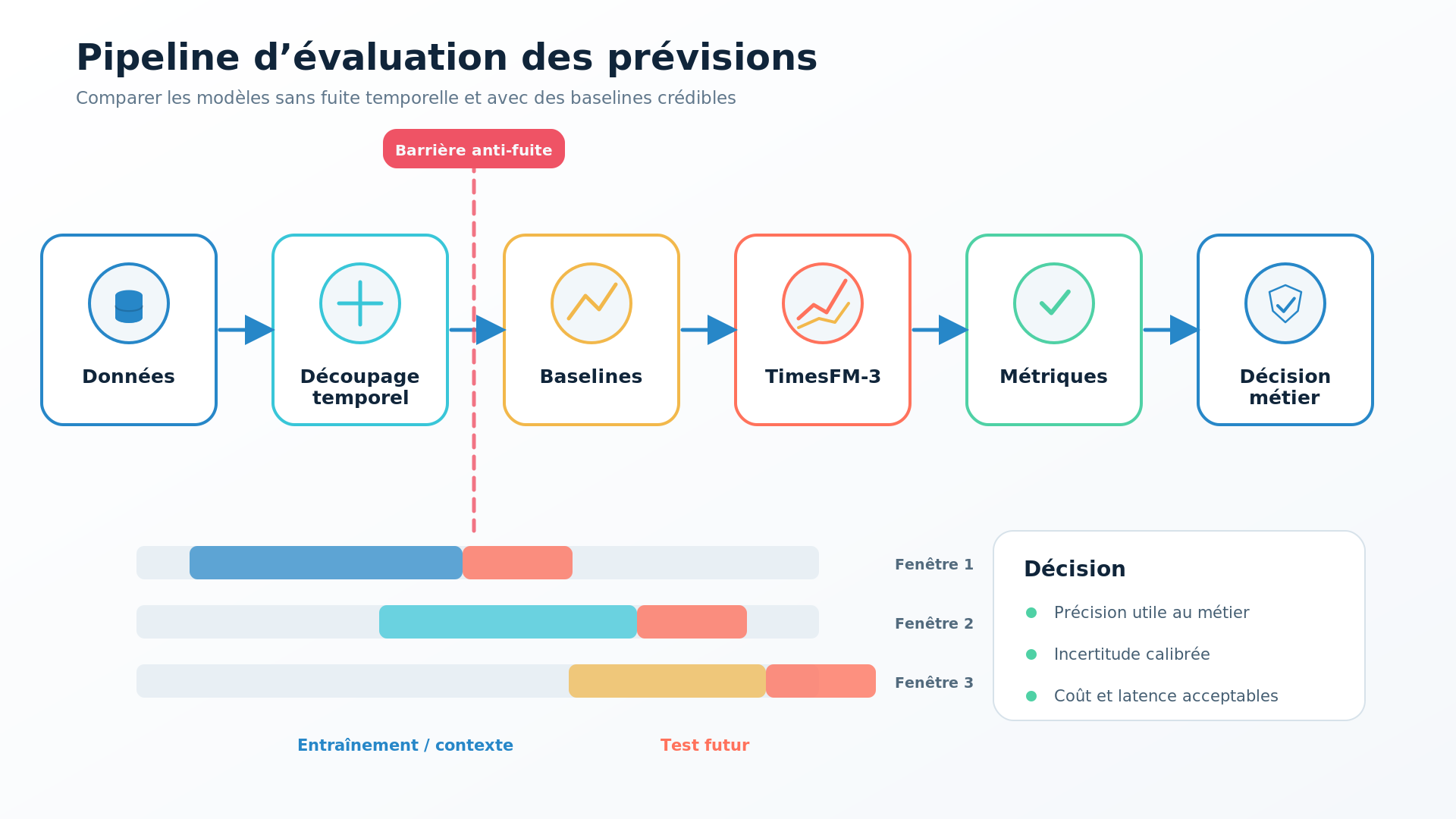
Temporal leakage is the most dangerous error in a forecasting project. It occurs when future information is used, directly or indirectly, to produce a prediction that is supposed to have been made in the past.
A classic example is promotional data recorded after a campaign but linked to its start date. A backtest run today then considers that the information was available, even though it was not available at decision time. The same issue applies to data corrections, aggregates calculated over a complete period, and variables updated retroactively.
Each column must have two dates: the event date and the availability date. The split uses the second one. For a forecast made on 1 June, the model receives only what was actually known on 1 June.
Normalization can also cause leakage if statistics are calculated over the entire dataset. Even when the model has its own normalization, business transformations, imputation, and series selection must be fitted only on the past of each window.
Finally, keep an untouched final test set. Repeatedly trying on the same horizon gradually turns that set into implicit training data for the team.
5. Building reliable backtesting
A single past/future split provides a fragile view. Use rolling-origin validation: choose several historical forecast dates, train or configure the methods with the data available at each date, and then measure the following horizon.
The windows should represent important situations: peak season, a quiet period, a launch, a supply disruption, and a change in trend. A model that performs well on average may fail precisely during the periods when the decision is most costly.
Compare at least four levels:
- a naïve baseline, such as the last value or the same period previously;
- a statistical method suited to seasonality;
- the solution currently used by the company;
- TimesFM-3 in univariate and multivariate modes when the data allows it.
The naïve baseline is essential. In many stable contexts, it remains difficult to beat. A model that slightly improves a benchmark but does not outperform “same day of the previous week” does not provide enough operational value.
Document the versions of the data, code, model, and dependencies. The result must be reproducible several months later, especially if a new model version changes the forecasts.
6. Measuring uncertainty, not just average error
Metrics must match the decision. MAE measures average absolute error and remains easy to read in business units. WAPE relates error to total volume, but can be dominated by large series. MASE compares the model with a naïve forecast and makes comparisons between series easier.
For quantiles, use a quantile loss and check calibration. If an interval announced at 80% contains the actual value only 50% of the time, uncertainty is underestimated. Conversely, a very wide interval covers almost everything but provides little decision support.
Add business metrics. Underforecasting stock can cost more than overforecasting it. A 10% error on a small item does not have the same impact as one on a strategic product. Calculate stockouts avoided, inventory tied up, scheduled hours, or reserved cloud budget.
Also evaluate stability. A forecast that changes sharply after a small input change can be difficult to use. Compare successive versions as new data arrives and measure how much the horizon is revised.
TimesFM-3’s probabilistic output is a potential advantage, provided that the quantiles are calibrated to the local context and actually used in decision rules.
7. Choosing between a foundation model, a specialized model, and a hybrid
A foundation model is suitable when the number of series is high, the startup time is short, and the organization wants a common base. It can also serve as a permanent challenger or a fallback solution when a specialized model lacks history.
A local model remains relevant when the phenomenon is highly specific, the variables are well controlled, and a few performance points have high value. It can incorporate business constraints, asymmetric cost functions, or a causal structure not represented in the general-purpose model.
The hybrid approach is often the most robust. TimesFM-3 provides a baseline forecast and quantiles; a business layer applies constraints, combines local information, or corrects an observed bias. Another model can be selected for certain series families.
The decision must include performance, cost, latency, licensing, confidentiality, explainability, and ease of operation. Also check the availability of announced integrations: as of 31 August 2026, Google indicated that TimesFM-3 was available on GitHub and Hugging Face, while BigQuery integration was announced for the following weeks.
8. A six-step pilot
Start with a scope where the decision and value are clear: twenty to one hundred series, a defined horizon, and an existing baseline. Avoid selecting only the cleanest series.
Second, build the variable availability table and remove leakage. Third, prepare five to ten backtest origins covering several business situations. Fourth, run all methods with the same protocol and the same data.
Fifth, organize a review with users. Present errors, intervals, and a few concrete cases without revealing the model name first, to reduce novelty bias. Ask which decision would have changed and with what impact.
Sixth, deploy in observation mode. The system generates forecasts, but the current method remains the decision-maker for several cycles. Measure quality, cost, stability, and availability before any switch.
Set success criteria before the test: minimum improvement over the baseline, acceptable calibration, maximum cost, execution time, and the proportion of series for which the model does not degrade the result. Without a prior threshold, the team will always find a way to justify the most recent model.
Conclusion
TimesFM-3 marks an interesting evolution in foundation models for time series: zero-shot multivariate forecasting, future-known variables, and probabilistic output in a single pass. These characteristics can reduce the entry cost and expand the number of series covered.
The value will nevertheless be demonstrated only by a local protocol, without temporal leakage, against strong baselines and with metrics connected to the business. Partitech supports data preparation, backtesting design, MLOps industrialization, and the translation of forecasts into measurable decisions.
References
- Google Research — “TimesFM-3: A zero-shot foundation model for multivariate forecasting”, 31 August 2026: https://research.google/blog/timesfm-3-a-zero-shot-foundation-model-for-multivariate-forecasting/
- Google Research — TimesFM repository: https://github.com/google-research/timesfm
- Hugging Face — TimesFM-3 model: https://huggingface.co/google/timesfm-3.0-pytorch